Regularized & Distributionally Robust Data-Enabled Predictive - PowerPoint PPT Presentation
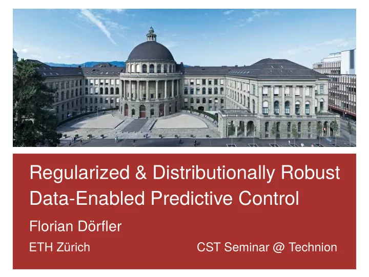
Regularized & Distributionally Robust Data-Enabled Predictive Control Florian D orfler ETH Z urich CST Seminar @ Technion Acknowledgements Jeremy Coulson Linbin Huang Paul Beuchat John Lygeros Ivan Markovsky Ezzat Elokda 1/30
Regularized & Distributionally Robust Data-Enabled Predictive Control Florian D¨ orfler ETH Z¨ urich CST Seminar @ Technion
Acknowledgements Jeremy Coulson Linbin Huang Paul Beuchat John Lygeros Ivan Markovsky Ezzat Elokda 1/30
Perspectives on model-based control model → models useful for system system x + = Ax + Bu system analysis, design, y = Cx + Du estimation, ... control → modeling from first principles & system ID controller From experiment design to closed-loop control � H˚ akan Hjalmarsson ∗ Department of Signals, Sensors and Systems, Royal Institute of Technology, S-100 44 Stockholm, Sweden recurring themes 1. Introduction be justified is for the commissioning of model predictive controllers. Ever increasing productivity demands and environmental It has also been recognized that models for control pose • modeling & system ID standards necessitate more and more advanced control meth- special considerations. Again quoting (Ogunnaike, 1996): ods to be employed in industry. However, such methods usu- “ There is abundant evidence in industrial practice that when modeling for control is not based on criteria related ally require a model of the process and modeling and system are very expensive identification are expensive. Quoting (Ogunnaike, 1996): to the actual end use , the results can sometimes be quite “ It is also widely recognized , however , that obtaining the disappointing. ” process model is the single most time consuming task in the Hence, efficient modeling and system identification tech- • models not always application of model-based control. ” niques suited for industrial use and tailored for control de- In Hussain (1999) it is reported that three quarters of the sign applications have become important enablers for indus- total costs associated with advanced control projects can trial advances. The Panel for Future Directions in Control, useful for control (Murray, ˚ Aström, Boyd, Brockett, & Stein, 2003), has iden- be attributed to modeling. It is estimated that models exist for far less than one percent of all processes in regulatory tified automatic synthesis of control algorithms , with inte- control. According to Desborough and Miller (2001), one of grated validation and verification as one of the major future • need for end-to-end the few instances when the cost of dynamic modeling can challenges in control. Quoting (Murray et al., 2003): “ Researchers need to develop much more powerful design tools that automate the entire control design process from automation solutions model development to hardware-in-the-loop simulation. ” 2/30
Control in a data-rich world • ever-growing trend in CS & applications: data-driven control by-passing models • canonical problem: black/gray-box u 2 y 2 system control based on I/O samples u 1 y 1 Q: Why give up physical modeling and reliable model-based algorithms ? data-driven control Data-driven control is viable alternative when • models are too complex to be useful Central promise: It (e.g., fluids, wind farms, & building automation) is often easier to learn • first-principle models are not conceivable control policies directly from data, rather than (e.g., human-in-the-loop, biology, & perception) learning a model. • modeling & system ID is too cumbersome Example: PID [˚ Astr¨ om, ’73] (e.g., robotics & electronics applications) 3/30
Snippets from the literature u 2 indirect data-driven control: y 2 sequential system ID + uncertainty u 1 y 1 quantification + robust control → recent end-to-end design pipelines with finite-sample guarantees + ? ø ID seeks best but not most useful model: “easier to learn policies ...” unknown system direct data-driven control: reinforcement learning / stochastic adaptive observation control / approximate dynamic programming action reinforcement learning control → spectacular theoretic & practical advances → more brute force storage/computation/data estimate ø not suitable for physical systems: reward real-time, safety-critical, continuous 4/30
Abstraction reveals pros & cons indirect data-driven control � � � minimize control cost x, u separation & outer � � certainty optimization subject to x, u satisfy state-space model equivalence � � � where x estimated from u, y & model middle opt. ( → LQG case) � � � u d , y d � no separation where model identified from data inner opt. ( → ID-4-control) → nested multi-level optimization problem direct data-driven control → trade-offs � � modular vs. end-2-end minimize control cost u, y suboptimal (?) vs. optimal � � � u d , y d � subject to u, y consistent with data convex vs. non-convex (?) Additionally: all above should be min-max or E ( · ) accounting for uncertainty ... 5/30
Colorful idea u 1 = 1 y 3 y 5 y 1 y 7 u 2 = u 3 = · · · = 0 x 0 =0 y 4 y 6 y 2 If you had the impulse response of a LTI system, then ... • can identify model (e.g., transfer function or Kalman-Ho realization) • or predictive control directly from raw data (dynamic matrix control) u future ( t ) u future ( t − 1) � � y future ( t ) = y 1 y 2 y 3 . . . · u future ( t − 2) . . . • insight : single trajectory generates all others — at least conceptually • today: can we do so with arbitrary, finite, and corrupted I/O samples ? 6/30
Contents I. Data-Enabled Predictive Control (DeePC): Basic Idea J. Coulson, J. Lygeros, and F. D¨ orfler. Data-Enabled Predictive Control: In the Shallows of the DeePC . arxiv.org/abs/1811.05890. II. From Heuristics & Numerical Promises to Theorems J. Coulson, J. Lygeros, and F. D ¨ orfler. Distributionally Robust Chance Constrained Data-enabled Predictive Control . https://arxiv.org/abs/2006.01702. III. Application: End-to-End Automation in Energy & Robotics L. Huang, J. Coulson, J. Lygeros, and F. D¨ orfler. Data-Driven Wide-Area Control . arxiv.org/abs/1911.12151. E. Elokda, J. Coulson, P. Beuchat, J. Lygeros, and F. D¨ orfler. Data-Enabled Predictive Control for Quadcopters . https://www.research-collection.ethz.ch/. [ click here ] for related publications
control Preview $- $. $/ $$ $, $0 $& !"#, 2;+B#& 2;+B#' !"#. 234*#$$5$, 234*#$-5$.5$ 234*#$.5$/5$ 234*#$05$& 234*#$,5$- 234*#$/5$0 !"#- !"#/ 234*#$%5$, 234*#$-5$.5% 234*#$.5$/5% 234*#$05$' $% $' ()*+#& ()*+#' 234*#$%5%1 complex 4-area power system : %1 large ( n =208 ), few sensors ( 8 ), uncontrolled flow (p.u.) 7;4:);<#!3=4+<> 6!758697 !:+:3;4#% nonlinear, noisy, stiff, input !&( !&' constraints, & decentralized !?>:*@ 234*#/5$/ A+):3:3;434= !&$ control specifications !&! 7;4:);<#!3=4+<> 6!758697 !:+:3;4#$ 10 ! " #! time (s) control objective: oscillation $1 234*#-5$1 - . / damping without model $ , 0 & !"#$ !"#& 234*#-5.5$ 234*#.5/5$ 234*#$5, 234*#05& 234*#/50 !"#% 234*#,5- !"#' (models are proprietary, grid has 234*#-5.5% 234*#.5/5% 234*#%5, 234*#05' % ' ()*+#$ 2;+B#$ 2;+B#% ()*+#% many owners, operation in flux, ...) control tie line flow (p.u.) !&( seek a method that works !&' reliably , can be efficiently !&$ implemented, & certifiable !&! → automating ourselves ! " #! #" $! $" %! !"#$%&'( collect data control 7/30
Behavioral view on LTI systems Definition: A discrete-time dynamical system is a 3 -tuple ( Z ≥ 0 , W , B ) where (i) Z ≥ 0 is the discrete-time axis, B is the set of (ii) W is a signal space, and all trajectories (iii) B ⊆ W Z ≥ 0 is the behavior. Definition: The dynamical system ( Z ≥ 0 , W , B ) is (i) linear if W is a vector space & B is a subspace of W Z ≥ 0 y (ii) and time-invariant if B ⊆ σ B , where σw t = w t +1 . u B = set of trajectories & B T is restriction to t ∈ [0 , T ] 8/30
LTI systems and matrix time series foundation of state-space subspace system ID & signal recovery algorithms u ( t ) y ( t ) y 3 u 4 y 4 u 1 u 3 y 1 u 7 y 5 y 7 t u 5 u 6 t y 2 u 2 y 6 � � [ b 0 a 0 b 1 a 1 ... b n a n ] spans left nullspace u ( t ) , y ( t ) satisfy recursive of Hankel matrix (collected from data) difference equation � � b 0 u t + b 1 u t +1 + . . . + b n u t + n + � u d �� u d �� u d � u d T − L +1 1 2 3 ··· y d y d y d y d a 0 y t + a 1 y t +1 + . . . + a n y t + n = 0 T − L +1 1 2 3 � u d �� u d �� u d � ⇒ ... . . 2 3 4 . � � y d y d y d (ARX / kernel representation) 2 3 4 u d � u d �� u d �� u d � = H L . ... y d . 3 4 5 . y d y d y d 3 4 5 ⇐ . . ... ... ... . . . . � u d � � u d � L T ··· ··· ··· under assumptions y d y d L T 9/30
Recommend
More recommend
Explore More Topics
Stay informed with curated content and fresh updates.
