Regression Given: Dataset D = { ( x i , Y i ) | i = 1 , ..., n } with - PowerPoint PPT Presentation

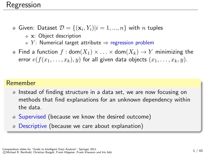
Regression Given: Dataset D = { ( x i , Y i ) | i = 1 , ..., n } with n tuples x : Object description Y : Numerical target attribute ⇒ regression problem Find a function f : dom ( X 1 ) × . . . × dom ( X k ) → Y minimizing the error e ( f ( x 1 , . . . , x k ) , y ) for all given data objects ( x 1 , . . . , x k , y ) . Remember Instead of finding structure in a data set, we are now focusing on methods that find explanations for an unknown dependency within the data. Supervised (because we know the desired outcome) Descriptive (because we care about explanation) Compendium slides for “Guide to Intelligent Data Analysis”, Springer 2011. 1 / 43 � Michael R. Berthold, Christian Borgelt, Frank H¨ c oppner, Frank Klawonn and Iris Ad¨ a

Regression line Given: A data set for two continuous attributes x and y . It is assumed that there is an approximate linear dependency between x and y : y ≈ a + bx Find a regression line (i.e. determine the parameters a and b ) such that the line fits the data as good as possible. Example Trend estimation (e.g. oil price over time) Epidemiology (e.g. cigarette smoking vs. lifespan ) Finance (e.g. return on investment vs. return on all risky assets) Economics (e.g. consumption vs. available income) Compendium slides for “Guide to Intelligent Data Analysis”, Springer 2011. 2 / 43 � Michael R. Berthold, Christian Borgelt, Frank H¨ c oppner, Frank Klawonn and Iris Ad¨ a

Regression Line y -distance Euclidean distance What is a good fit? Compendium slides for “Guide to Intelligent Data Analysis”, Springer 2011. 3 / 43 � Michael R. Berthold, Christian Borgelt, Frank H¨ c oppner, Frank Klawonn and Iris Ad¨ a

Cost functions Usually, the sum of square errors in y -direction is chosen as cost function (to be minimized). Other reasonable cost functions: mean absolute distance in y -direction mean Euclidean distance maximum absolute distance in y -direction (or equivalently: the maximum squared distance in y -direction) maximum Euclidean distance . . . Compendium slides for “Guide to Intelligent Data Analysis”, Springer 2011. 4 / 43 � Michael R. Berthold, Christian Borgelt, Frank H¨ c oppner, Frank Klawonn and Iris Ad¨ a

Construction Given data ( x i , y i ) ( i = 1 , . . . , n ), the least squares cost function is n (( a + bx i ) − y i ) 2 . � F ( a, b ) = i =1 Goal The y-values that are computed with the linear equation should (in total) deviate as little as possible from the measured values. Compendium slides for “Guide to Intelligent Data Analysis”, Springer 2011. 5 / 43 � Michael R. Berthold, Christian Borgelt, Frank H¨ c oppner, Frank Klawonn and Iris Ad¨ a

Finding the minimum A necessary condition for a minimum of the cost function i =1 (( a + bx i ) − y i ) 2 is that the partial derivatives of this F ( a, b ) = � n function w.r.t the parameters a and b vanish, that is n n ∂F ∂F � � ∂a = 2( a + bx i − y i ) = 0 and ∂b = 2( a + bx i − y i ) x i = 0 i =1 i =1 As a consequence, we obtain the so-called normal equations � n � n � n � n � � n � � � � x 2 � na + x i b = y i and x i a + b = x i y i i i =1 i =1 i =1 i =1 i =1 that is, a two-equation system with two unknowns a and b which has a unique solution (if at least two different x -values exist). Compendium slides for “Guide to Intelligent Data Analysis”, Springer 2011. 6 / 43 � Michael R. Berthold, Christian Borgelt, Frank H¨ c oppner, Frank Klawonn and Iris Ad¨ a

Least squares and MLE A regression line can be interpreted as a maximum likelihood estimator (MLE): Assumption: The data generation process can be described well by the model y = a + bx + ξ, where ξ is normally distributed random variable with mean 0 and (unknown) variance σ 2 . The parameter that minimizes the sum of squared deviations (in y -direction) from the data points maximizes the probability of the data given this model class. Compendium slides for “Guide to Intelligent Data Analysis”, Springer 2011. 7 / 43 � Michael R. Berthold, Christian Borgelt, Frank H¨ c oppner, Frank Klawonn and Iris Ad¨ a

Least squares and MLE Therefore, − ( y − ( a + bx )) 2 1 � � f ( y | x ) = √ 2 πσ 2 · exp , 2 σ 2 leading to the likelihood function L (( x 1 , y 1 ) , . . . ( x n , y n ); a, b, σ 2 ) n � = f ( y i | x i ) i =1 n − ( y i − ( a + bx i )) 2 � � 1 � = · √ 2 πσ 2 · exp . 2 σ 2 i =1 Compendium slides for “Guide to Intelligent Data Analysis”, Springer 2011. 8 / 43 � Michael R. Berthold, Christian Borgelt, Frank H¨ c oppner, Frank Klawonn and Iris Ad¨ a

Least squares and MLE To simplify the computation of derivatives for finding the maximum, we compute the logarithm: ln L (( x 1 , y 1 ) , . . . ( x n , y n ); a, b, σ 2 ) n − ( y i − ( a + bx i )) 2 � � 1 � = ln √ 2 πσ 2 · exp 2 σ 2 i =1 n n 1 1 � � ( y i − ( a + bx i )) 2 = ln √ 2 πσ 2 − 2 σ 2 i =1 i =1 Compendium slides for “Guide to Intelligent Data Analysis”, Springer 2011. 9 / 43 � Michael R. Berthold, Christian Borgelt, Frank H¨ c oppner, Frank Klawonn and Iris Ad¨ a

Least squares and MLE n n 1 1 � � ( y i − ( a + bx i )) 2 ln √ 2 πσ 2 − 2 σ 2 i =1 i =1 From this expression it becomes clear by computing the derivatives w.r.t. the parameters a and b that maximizing the likelihood function is equivalent to minimizing n � ( y i − ( a + bx i )) 2 . F ( a, b ) = i =1 Compendium slides for “Guide to Intelligent Data Analysis”, Springer 2011. 10 / 43 � Michael R. Berthold, Christian Borgelt, Frank H¨ c oppner, Frank Klawonn and Iris Ad¨ a

Regression polynomials The least squares method can be extended to regression polynomials (e.g. x = time, y = distance by constant acceleration) y = p ( x ) = a 0 + a 1 x + . . . + a m x m with a given fixed degree m . We have to minimize the error function n � ( p ( x i ) − y i ) 2 F ( a 0 , . . . , a m ) = i =1 n � i ) − y i ) 2 (( a 0 + a 1 x i + . . . + a m x m = i =1 In analogy to the linear case, we form the partial derivatives of this function w.r.t. the parameters a k , 0 ≤ k ≤ m , and equate them to zero. Compendium slides for “Guide to Intelligent Data Analysis”, Springer 2011. 11 / 43 � Michael R. Berthold, Christian Borgelt, Frank H¨ c oppner, Frank Klawonn and Iris Ad¨ a

Multilinear regression Given: A data set (( x 1 , y 1 ) , . . . , ( x n , y n )) with input vectors x i and corresponding responses y i , 1 ≤ i ≤ n . for which we want to determine the linear regression function m � y = f ( x 1 , . . . , x m ) = a 0 + a k x k . k =1 Example Price of a house depending on its size ( x 1 ) and age ( x 2 ) Ice cream consumption based on the temperature ( x 1 ), the price ( x 2 ) and the family income ( x 3 ) Electric consumption based on the number of flats with one ( x 1 ), two ( x 2 ), three ( x 3 ) and four or more persons ( x 4 ) living in them Compendium slides for “Guide to Intelligent Data Analysis”, Springer 2011. 12 / 43 � Michael R. Berthold, Christian Borgelt, Frank H¨ c oppner, Frank Klawonn and Iris Ad¨ a

Multilinear regression n � ( f ( x i ) − y i ) 2 F ( a 0 , . . . , a m ) = i =1 n � 2 � a 0 + a 1 x ( i ) � 1 + . . . + a m x ( i ) = m − y i i =1 In order to derive the normal equations, it is convenient to write the functional to minimize in matrix form F ( a ) = ( Xa − y ) ⊤ ( Xa − y ) where       a 0 1 x 1 , 1 · · · x 1 ,m y 1 . . . . . ... . . . . . a =  , X =  and y =       . . . . .     a m 1 x n, 1 · · · x n,m y n Compendium slides for “Guide to Intelligent Data Analysis”, Springer 2011. 13 / 43 � Michael R. Berthold, Christian Borgelt, Frank H¨ c oppner, Frank Klawonn and Iris Ad¨ a

Multilinear regression Again a necessary condition for a minimum is that the partial derivatives of this function w.r.t the coefficients a k , 0 ≤ k ≤ m , vanish. Using the differential operator ∇ , we can write these conditions as � ∂ ∇ a F ( a ) = d F ( a ) , ∂ ∂ � d a F ( a ) = F ( a ) , . . . , F ( a ) = 0 ∂a 0 ∂a 1 ∂a m Whereas the differential operator behaves like a vector � ∂ , ∂ ∂ � ∇ a = , . . . , ∂a 0 ∂a 1 ∂a m Compendium slides for “Guide to Intelligent Data Analysis”, Springer 2011. 14 / 43 � Michael R. Berthold, Christian Borgelt, Frank H¨ c oppner, Frank Klawonn and Iris Ad¨ a

Multilinear regression F ( a ) = ( Xa − y ) ⊤ ( Xa − y ) to find the minimum we use the differential operator ∇ ∇ a ( Xa − y ) ⊤ ( Xa − y ) 0 = � ⊤ ( ∇ a ( Xa − y )) ⊤ ( Xa − y ) + � ( Xa − y ) ⊤ ( ∇ a ( Xa − y )) = ( ∇ a ( Xa − y )) ⊤ ( Xa − y ) + ( ∇ a ( Xa − y )) ⊤ ( Xa − y ) = 2 X ⊤ ( Xa − y ) = 2 X ⊤ Xa − 2 X ⊤ y = from which we obtain the system of normal equations X ⊤ Xa = X ⊤ y . Compendium slides for “Guide to Intelligent Data Analysis”, Springer 2011. 15 / 43 � Michael R. Berthold, Christian Borgelt, Frank H¨ c oppner, Frank Klawonn and Iris Ad¨ a