Reduced models and the bottlenecks for problems with many parameters - PowerPoint PPT Presentation

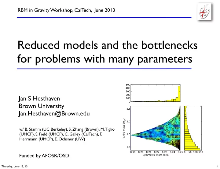
RBM in Gravity Workshop, CalTech, June 2013 Reduced models and the bottlenecks for problems with many parameters Jan S Hesthaven Brown University Jan.Hesthaven@Brown.edu w/ B. Stamm (UC Berkeley), S. Zhang (Brown), M. Tiglio (UMCP), S. Field (UMCP), C. Galley (CalTech), F. Herrmann (UMCP), E. Ochsner (UW) Funded by AFOSR/OSD Thursday, June 13, 13 1

Basic questions to consider Reduced models WHAT do we mean by ‘reduced models’ ? WHY should we care ? WHEN could it work ? HOW do we know ? DOES it work ? WHEN do problems arise ? Thursday, June 13, 13 2

Reduced models ? We do not consider reduced physics - High-frequency vs low-frequency EM vs � � � � E + ω 2 E = f �� 2 E = f Viscous vs inviscid fluid flows ∂ u ∂ u ∂ t + u · � u = �� p + ν � 2 u ∂ t + u · � u = �� p vs � · u = 0 � · u = 0 .. but reduced representations of the full problem Thursday, June 13, 13 3

.. but WHY ? Assume we are interested in �� 2 u ( x , µ ) = f ( x , µ ) x ∈ Ω and wish to solve it accurately for many values of ‘some’ parameter µ We can use our favorite numerical method A h u h ( x , µ ) = f h ( x , µ ) dim( u h ) = N � 1 For many parameter values, this is expensive - and slow ! Thursday, June 13, 13 4

.. but WHY (con’t) Assume we (somehow) know V T V = I u h ( x , µ ) � u RB ( x , µ ) = V a ( µ ) dim( V ) = N × N dim( a ) = N Then we can recover a solution for a new parameter as little cost (V T A h V)V T u h ( µ ) = V T f h ( µ ) .. if this behaves ! N × N N N Thursday, June 13, 13 5

.. but WHY (con’t) So IF ‣ .. we know the orthonormal basis - V ‣ .. and it allows an accurate representation - u RB ( µ ) ‣ .. and we can evaluate RHS ‘fast’- O ( N ) we can evaluate new solutions at cost - O ( N ) So WHY ? - a promise to do more with less Thursday, June 13, 13 6

Model reduction We seek an accurate way to evaluate the solution at new parameter values at reduced complexity. input: parameter value µ ∈ D PDE solver L h ( u h ( µ ); µ ) = 0 output: s h ( µ ) = l ( u h ( µ ); µ ) Thursday, June 13, 13 7

When is that relevant ? Examples in many CSE application domains ‣ Optimization/inversion/control problems ‣ Simulation based data bases ‣ Uncertainty quantification ‣ Sub-scale models in multi-scale modeling ‣ In-situ/deployed modeling D. Knezevic et al, 2010 Thursday, June 13, 13 8

When does this work ? For this to be successful there must be some structure to the solution under parameter variation Assumption : The solution varies smoothly on a low- dimensional manifold under parameter variation. M Choosing the samples well, we should be able to derive good approximations for all u ( µ j ) u ( µ ) parameters X Thursday, June 13, 13 9

Check the assumption Two dimensional parameterization with polar angle and frequency rs : ( k, θ ) ∈ [1 , 25] × [0 , π ], φ is fixed. Geometry : 0.1 0.01 0.001 0.0001 0.00001 1 x 10 -6 z 1 x 10 -7 1 x 10 -8 θ 1 x 10 -9 1 x 10 -10 y 1 x 10 -11 x 1 x 10 -12 1 x 10 -13 1 x 10 -14 1 x 10 -15 φ 1 x 10 -16 1 x 10 -17 0 500 1000 1500 2000 2500 3000 singular values With 200 basis functions you can reach a precision of 1e-7! Thursday, June 13, 13 10

Reduced basis method Low dimensional representations may exists for many - but not all - problems. Of course not a new observation - ‣ KL-expansions/POD etc ‣ Computes basis through SVD ‣ Costly ‣ Error ? ‣ Krylov based methods ‣ Computes basis through Krylov subspace ‣ Error ? Let’s consider a different approach Thursday, June 13, 13 11

A second look We consider physical systems of the form L ( x , µ ) u ( x , µ ) = f ( x , µ ) x ∈ Ω u ( x , µ ) = g ( x , µ ) x ∈ ∂ Ω where the solutions are implicitly parameterized by µ ∈ D ⊂ R M ‣ How do we find the basis. ‣ How do we ensure accuracy under parameter variation ? ‣ What about speed ? Thursday, June 13, 13 12

The truth Let us define: The exact solution: Find such that u ( µ ) ∈ X a ( u, µ, v ) = f ( µ, v ) , ∀ v ∈ X The truth solution: Find such that u h ( µ ) ∈ X h dim( X h ) = N a h ( u h , µ, v h ) = f h ( µ, v h ) , ∀ v h ∈ X h The RB solution: Find such that u RB ( µ ) ∈ X N a h ( u RB , µ, v N ) = f h ( µ, v N ) , ∀ v N ∈ X N dim( X N ) = N We always assume that N � N Thursday, June 13, 13 13

The truth and errors Solving for the truth is expensive - but we need to be able to trust the RB solution � u ( µ ) � u RB ( µ ) � � � u ( µ ) � u h ( µ ) � + � u h ( µ ) � u RB ( µ ) � We assume that � u ( µ ) � u h ( µ ) � � ε This is your favorite solver and it is assumed it can be as accurate as you desire - the truth Bounding we achieve two things ‣ Ability to build a basis at minimal cost ‣ Certify the quality of the model Thursday, June 13, 13 14

The error estimate Consider the discrete truth problem A( µ ) u h ( µ ) = f h ( µ ) Express the solution as u h ∈ X h u h = u N + u ⊥ u N ∈ X N This results in the truth problem � A 1 , 1 � � u N � f RB � � A 1 , 2 = A 2 , 1 A 2 , 2 u ⊥ f ⊥ as well as the reduced problem A 1 , 1 u RB = f RB Thursday, June 13, 13 15

The error estimate This yields the estimate for the error � A 1 , 1 � � u N − u RB � � � A 1 , 2 0 = A 2 , 1 A 2 , 2 u ⊥ f ⊥ − A 2 , 1 u RB We can recognize the right hand side as � f RB − A 1 , 1 u RB � � � 0 = = f h − Au RB = R ( µ ) f ⊥ − A 2 , 1 u RB f ⊥ − A 2 , 1 u RB and we recover � u h ( µ ) � u RB ( µ ) � � � A − 1 ( µ ) �� R ( µ ) � So with the residual and an estimate of the norm of the inverse of A we can bound the error Thursday, June 13, 13 16

RBM 101 We use the error estimator to construct the reduced basis in a greedy approach.  1. Define a (fine)training set in parameter space Π train  2. Choose a member randomly and solve truth.  3. Define  u RB = u h ( µ 1 ) a. Find µ i +1 = arg sup ε N ( µ )  µ ∈ Π train b. Compute u h ( µ i +1 )  c. Orthonormalize wrt u RB   d. Add new solution basis      4. Continue until ε N ≤ ε       sup  µ ∈ Π train N � u i Resulting in u RM ( µ ) = N ( µ ) ξ i i =1 Thursday, June 13, 13 17

2D Pacman problem Scattering by 2D PEC Pacman Backscatter depends very sensitively on cutout angle and frequency. 30 Cylinder WedgeAngle = 18.5 Deg 20 WedgeAngle = 21.5 Deg 10 0 Difference in scattering is clear in fields − 10 − 20 0 1 2 3 4 5 6 TM polarization Thursday, June 13, 13 18

2D Pacman problem 15 Greedy approach selects 10 critical angles early in the 5 selection process 0 − 5 Parameter is gap angle − 10 − 15 9.6 11.6 14.3 18.5 21.5 15 10 5 Convergence of output with 0 O(10) basis elements − 5 Truth RB with 9 Bases − 10 RB with 11 Bases − 15 9.6 11.6 14.3 18.5 21.5 Output of interest - backscatter Thursday, June 13, 13 19

2D Pacman problem 40 Convergence of error bounds over full parameter range 20 0 − 20 RB output with 13 bases Output + error estimate Output − error estimate − 40 Exponential convergence of 9.6 11.6 14.3 18.5 21.5 12 predicted error estimator and RB output with 15 bases 10 Output + error estimate real error over large training set Output − error estimate 8 6 4 Worst Case RBM Error Worst Case Error Estimate Error/Error Estimate 2 0 10 0 − 2 9.6 11.6 14.3 18.5 21.5 12 − 5 RB output with 17 bases 10 Output + error estimate 10 Output − error estimate 8 6 5 10 15 20 25 30 Number of Bases 4 2 0 9.6 11.6 14.3 18.5 21.5 Thursday, June 13, 13 20

RBM for wave catalogs The challenge is .. use a solver to predict wave forms .. repeat for many parameter values to build catalog We shall consider the construction of a reduced basis based on a greedy approach Goal: Seek a finite dimensional basis og C N = { Ψ i } N i =1 . Ψ i ≡ h � µ = � µ i d N ( H ) = min C N max u ∈ W N || u − h � min µ || . � µ Thursday, June 13, 13 21

RBM for wave catalogs The algorithm for this is Algorithm 1 Greedy algorithm for building a reduced basis space 1: Input: training space Ξ and waveforms sampled at training space H Ξ 2: Randomly select some � µ 1 ∈ Ξ 3: C 1 = { h � µ 1 } 4: N = 1 5: ε = 1 � We use normalized waveforms 6: while ε ≥ Tolerance do µ ∈ Ξ do for � 7: Compute Err( � µ ) = || h � µ − P N ( h � µ ) || 8: end for 9: Choose µ N +1 = arg max � µ ∈ Ξ Err( � µ ) � 10: C N +1 = { h � µ N +1 } µ 1 , ..., h � µ N , h � 11: ε = Err( � µ N +1 ) 12: N = N + 1 13: 14: end while 15: ε N = ε 16: Output: Greedy error ε N , C N , representations P N ( h � µ ) ∈ W N = span ( C N ) Thursday, June 13, 13 22

RBM for wave catalogs Test case is BNS inspiral for LIGO. Analytic wave form with 2 parameters Thursday, June 13, 13 23

RBM for wave catalogs RBM sample points for two-parameter problem Thursday, June 13, 13 24