Recurrent Networks Part 3 1 Y(t+6) Story so far Stock vector - PowerPoint PPT Presentation

Deep Learning Recurrent Networks Part 3 1

Y(t+6) Story so far Stock vector X(t) X(t+1) X(t+2) X(t+3) X(t+4) X(t+5) X(t+6) X(t+7) • Iterated structures are good for analyzing time series data with short-time dependence on the past – These are “ Time delay ” neural nets, AKA convnets • Recurrent structures are good for analyzing time series data with long-term dependence on the past – These are recurrent neural networks 2

Story so far Y(t) h -1 X(t) t=0 Time • Iterated structures are good for analyzing time series data with short-time dependence on the past – These are “Time delay” neural nets, AKA convnets • Recurrent structures are good for analyzing time series data with long-term dependence on the past – These are recurrent neural networks 3

Recap: Recurrent networks can be incredibly effective at modeling long-term dependencies 4

Recurrent structures can do what static structures cannot 1 0 1 0 1 0 1 1 1 1 0 1 Previous Carry RNN unit MLP carry out 1 0 1 0 0 0 1 1 0 0 1 0 1 1 0 0 1 0 1 1 0 0 • The addition problem: Add two N-bit numbers to produce a N+1-bit number – Input is binary – Will require large number of training instances • Output must be specified for every pair of inputs • Weights that generalize will make errors – Network trained for N-bit numbers will not work for N+1 bit numbers • An RNN learns to do this very quickly – With very little training data! 5

Story so far Y desired (t) DIVERGENCE Y(t) h -1 X(t) t=0 Time • Recurrent structures can be trained by minimizing the divergence between the sequence of outputs and the sequence of desired outputs – Through gradient descent and backpropagation 6

Story so far Primary topic for today Y desired (t) DIVERGENCE Y(t) h -1 X(t) t=0 Time • Recurrent structures can be trained by minimizing the divergence between the sequence of outputs and the sequence of desired outputs – Through gradient descent and backpropagation 7

Story so far: stability • Recurrent networks can be unstable – And not very good at remembering at other times sigmoid tanh relu 8

Vanishing gradient examples.. ELU activation, Batch gradients Input layer Output layer • Learning is difficult: gradients tend to vanish.. 9

The long-term dependency problem 1 PATTERN1 […………………………..] PATTERN 2 Jane had a quick lunch in the bistro. Then she.. • Long-term dependencies are hard to learn in a network where memory behavior is an untriggered function of the network – Need it to be a triggered response to input 10

Long Short-Term Memory • The LSTM addresses the problem of input- dependent memory behavior 11

LSTM-based architecture Y(t) X(t) Time • LSTM based architectures are identical to RNN-based architectures 12

Bidirectional LSTM Y(0) Y(1) Y(2) Y(T-2) Y(T-1) Y(T) h f (-1) X(0) X(1) X(2) X(T-2) X(T-1) X(T) h b (inf) X(0) X(1) X(2) X(T-2) X(T-1) X(T) t • Bidirectional version.. 13

Key Issue Primary topic for today Y desired (t) DIVERGENCE Y(t) h -1 X(t) t=0 Time • How do we define the divergence • Also: how do we compute the outputs.. 14

What follows in this series on recurrent nets • Architectures: How to train recurrent networks of different architectures • Synchrony: How to train recurrent networks when – The target output is time-synchronous with the input – The target output is order-synchronous, but not time synchronous – Applies to only some types of nets • How to make predictions/inference with such networks 15

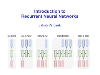
Variants on recurrent nets Images from Karpathy • Conventional MLP • Time-synchronous outputs – E.g. part of speech tagging 16

Variants on recurrent nets • Sequence classification: Classifying a full input sequence – E.g phoneme recognition • Order synchronous , time asynchronous sequence-to-sequence generation – E.g. speech recognition – Exact location of output is unknown a priori 17

Variants Images from Karpathy • A posteriori sequence to sequence: Generate output sequence after processing input – E.g. language translation • Single-input a posteriori sequence generation – E.g. captioning an image 18

Variants on recurrent nets Images from Karpathy • Conventional MLP • Time-synchronous outputs – E.g. part of speech tagging 19

Regular MLP for processing sequences Y(t) X(t) t=0 Time • No recurrence in model – Exactly as many outputs as inputs – Every input produces a unique output – The output at time 𝑢 is unrelated to the output at 𝑢′ ≠ 𝑢 20

Learning in a Regular MLP Y desired (t) DIVERGENCE Y(t) X(t) t=0 Time • No recurrence – Exactly as many outputs as inputs • One to one correspondence between desired output and actual output – The output at time 𝑢 is unrelated to the output at 𝑢′ ≠ 𝑢 . 21

Regular MLP Y target (t) DIVERGENCE Y(t) • Gradient backpropagated at each time 𝛼 𝑍(𝑢) 𝐸𝑗𝑤 𝑍 𝑢𝑏𝑠𝑕𝑓𝑢 1 … 𝑈 , 𝑍(1 … 𝑈) • Common assumption: 𝐸𝑗𝑤 𝑍 𝑢𝑏𝑠𝑕𝑓𝑢 1 … 𝑈 , 𝑍(1 … 𝑈) = ෍ 𝑥 𝑢 𝐸𝑗𝑤 𝑍 𝑢𝑏𝑠𝑕𝑓𝑢 𝑢 , 𝑍(𝑢) 𝑢 𝛼 𝑍(𝑢) 𝐸𝑗𝑤 𝑍 𝑢𝑏𝑠𝑕𝑓𝑢 1 … 𝑈 , 𝑍(1 … 𝑈) = 𝑥 𝑢 𝛼 𝑍(𝑢) 𝐸𝑗𝑤 𝑍 𝑢𝑏𝑠𝑕𝑓𝑢 𝑢 , 𝑍(𝑢) – 𝑥 𝑢 is typically set to 1.0 – This is further backpropagated to update weights etc 22

Regular MLP Y target (t) DIVERGENCE Y(t) • Gradient backpropagated at each time 𝛼 𝑍(𝑢) 𝐸𝑗𝑤 𝑍 𝑢𝑏𝑠𝑕𝑓𝑢 1 … 𝑈 , 𝑍(1 … 𝑈) • Common assumption: 𝐸𝑗𝑤 𝑍 𝑢𝑏𝑠𝑕𝑓𝑢 1 … 𝑈 , 𝑍(1 … 𝑈) = ෍ 𝐸𝑗𝑤 𝑍 𝑢𝑏𝑠𝑕𝑓𝑢 𝑢 , 𝑍(𝑢) 𝑢 𝛼 𝑍(𝑢) 𝐸𝑗𝑤 𝑍 𝑢𝑏𝑠𝑕𝑓𝑢 1 … 𝑈 , 𝑍(1 … 𝑈) = 𝛼 𝑍(𝑢) 𝐸𝑗𝑤 𝑍 𝑢𝑏𝑠𝑕𝑓𝑢 𝑢 , 𝑍(𝑢) – This is further backpropagated to update weights etc Typical Divergence for classification: 𝐸𝑗𝑤 𝑍 𝑢𝑏𝑠𝑕𝑓𝑢 𝑢 , 𝑍(𝑢) = 𝑌𝑓𝑜𝑢(𝑍 𝑢𝑏𝑠𝑕𝑓𝑢 , 𝑍) 23

Variants on recurrent nets Images from Karpathy • Conventional MLP • Time-synchronous outputs – E.g. part of speech tagging 24

Variants on recurrent nets Images from Karpathy With a brief detour into modelling language • Conventional MLP • Time-synchronous outputs – E.g. part of speech tagging 25

Time synchronous network CD NNS VBD IN DT JJ NN h -1 two roads diverged in a yellow wood • Network produces one output for each input – With one-to-one correspondence – E.g. Assigning grammar tags to words • May require a bidirectional network to consider both past and future words in the sentence 26

Time-synchronous networks: Inference Y(0) Y(1) Y(2) Y(T-2) Y(T-1) Y(T) h -1 X(0) X(1) X(2) X(T-2) X(T-1) X(T) • Process input left to right and produce output after each input 27

Time-synchronous networks: Inference Y(0) Y(1) Y(2) Y(T-2) Y(T-1) Y(T) h -1 X(0) X(1) X(2) X(T-2) X(T-1) X(T) X(0) X(1) X(2) X(T-2) X(T-1) X(T) • For bidirectional networks: – Process input left to right using forward net – Process it right to left using backward net – The combined outputs are used subsequently to produce one output per input symbol • Rest of the lecture(s) will not specifically consider bidirectional nets, but the discussion generalizes 28

How do we train the network Y(0) Y(1) Y(2) Y(T-2) Y(T-1) Y(T) h -1 X(0) X(1) X(2) X(T-2) X(T-1) X(T) t • Back propagation through time (BPTT) • Given a collection of sequence training instances comprising input sequences and output sequences of equal length, with one-to-one correspondence – (𝐘 𝑗 , 𝐄 𝑗 ) , where – 𝐘 𝑗 = 𝑌 𝑗,0 , … , 𝑌 𝑗,𝑈 – 𝐄 𝑗 = 𝐸 𝑗,0 , … , 𝐸 𝑗,𝑈 29

Training: Forward pass Y(0) Y(1) Y(2) Y(T-2) Y(T-1) Y(T) h -1 X(0) X(1) X(2) X(T-2) X(T-1) X(T) t • For each training input: • Forward pass: pass the entire data sequence through the network, generate outputs 30

Training: Computing gradients Y(0) Y(1) Y(2) Y(T-2) Y(T-1) Y(T) h -1 X(0) X(1) X(2) X(T-2) X(T-1) X(T) t • For each training input: • Backward pass: Compute gradients via backpropagation – Back Propagation Through Time 31

Back Propagation Through Time 𝐸𝐽𝑊 𝐸(1. . 𝑈) 𝑍(0) 𝑍(1) 𝑍(2) 𝑍(𝑈 − 2) 𝑍(𝑈 − 1) 𝑍(𝑈) h -1 𝑌(0) 𝑌(1) 𝑌(2) 𝑌(𝑈 − 2) 𝑌(𝑈 − 1) 𝑌(𝑈) • The divergence computed is between the sequence of outputs by the network and the desired sequence of outputs • This is not just the sum of the divergences at individual times  Unless we explicitly define it that way 32

Back Propagation Through Time 𝐸𝐽𝑊 𝐸(1. . 𝑈) 𝑍(0) 𝑍(1) 𝑍(2) 𝑍(𝑈 − 2) 𝑍(𝑈 − 1) 𝑍(𝑈) h -1 𝑌(0) 𝑌(1) 𝑌(2) 𝑌(𝑈 − 2) 𝑌(𝑈 − 1) 𝑌(𝑈) First step of backprop: Compute 𝛼 𝑍(𝑢) 𝐸𝐽𝑊 for all t The rest of backprop continues from there 33