Recognition Part I CSE 576 What we have seen so far: Vision as - PowerPoint PPT Presentation
Recognition Part I CSE 576 What we have seen so far: Vision as Measurement Device Real-time stereo on Mars Physics-based Vision Virtualized Reality Structure from Motion Slide Credit: Alyosha Efros Visual Recognition What does it mean
Estimating Parameters Maximum likelihood estimates: Mean: jth training example Variance: =1 if x true, else 0
another probabilistic approach!!! Naïve Bayes: directly estimate the data distribution P(X,Y)! • challenging due to size of distribution! • make Naïve Bayes assumption: only need P(X i |Y)! But wait, we classify according to: • max Y P(Y|X) Why not learn P(Y|X) directly?
Discriminative vs. generative • Generative model 0.1 ( The artist ) 0.05 0 0 10 20 30 40 50 60 70 x = data • Discriminative model 1 (The lousy painter) 0.5 0 0 10 20 30 40 50 60 70 x = data • Classification function 1 -1 0 10 20 30 40 50 60 70 80 x = data
Logistic Regression Logistic function (Sigmoid): Learn P(Y| X ) directly! • • Assume a particular functional form • Sigmoid applied to a linear function of the data: Z 1 P ( Y = 1 | X ) = 1 + exp ( w 0 + ∑ n i = 1 w i X i ) exp ( w 0 + ∑ n i = 1 w i X i ) P ( Y = 0 | X ) = 1 + exp ( w 0 + ∑ n i = 1 w i X i )
Logistic Regression: decision boundary 1 exp ( w 0 + ∑ n i = 1 w i X i ) P ( Y = 1 | X ) = P ( Y = 0 | X ) = 1 + exp ( w 0 + ∑ n i = 1 w i X i ) 1 + exp ( w 0 + ∑ n i = 1 w i X i ) • Prediction: Output the Y with highest P(Y|X) – For binary Y, output Y=0 if w.X+w 0 = 0 1 < P ( Y = 0 | X ) P ( Y = 1 | X ) n ∑ 1 < exp ( w 0 + w i X i ) i = 1 n ∑ 0 < w 0 + w i X i i = 1 A Linear Classifier!
Loss functions / Learning Objectives: Likelihood v. Conditional Likelihood Generative (Naïve Bayes) Loss function: Data likelihood But, discriminative (logistic regression) loss function: Conditional Data Likelihood • Doesn’t waste effort learning P(X) – focuses on P(Y| X ) all that matters for classification • Discriminative models cannot compute P( x j | w )!
Conditional Log Likelihood equal because y j is in {0,1} ⇤ remaining steps: substitute definitions, expand logs, and simplify e w 0 + P i w i X i 1 y j ln ⇤ i w i X i + (1 − y j ) ln = 1 + e w 0 + P 1 + e w 0 + P i w i X i j
Logistic Regression Parameter Estimation: Maximize Conditional Log Likelihood Good news: l ( w ) is concave function of w → no locally optimal solutions! Bad news: no closed-form solution to maximize l ( w ) Good news: concave functions “easy” to optimize
Optimizing concave function – Gradient ascent Conditional likelihood for Logistic Regression is concave ! Gradient: Update rule: Gradient ascent is simplest of optimization approaches • e.g., Conjugate gradient ascent much better
Maximize Conditional Log Likelihood: Gradient ascent ⌥ � ⇥ ⇧ ⇤ ⌅⌃ � ∂ l ( w ) ∂ i ) − ∂ ⌥ ⌥ w i x j ⌥ w i x j ∂ wy j ( w 0 + = ∂ w ln 1 + exp( w 0 + i ) = ∂ w i j i i ⇧ ⌃ i − x j i w i x j i exp( w 0 + ⌥ i ) � � y j x j ⌥ = i w i x j ⌥ 1 + exp( w 0 + ⌥ i ) j ⇧ ⌃ i w i x j ⇧ ⌃ exp( w 0 + ⌥ i ) � x j y j − = i i w i x j 1 + exp( w 0 + ⌥ i ) P j ∂ l ( w ) y j − P ( Y j = 1 | x j , w ) � x j � ⇥ = i ∂ w i j ⇧ ⇤
Gradient ascent for LR Gradient ascent algorithm: (learning rate η > 0) do: For i=1…n: (iterate over weights) until “change” < e Loop over training examples!
⌥ 1 Large parameters … 1 + e − ax Result : 1.0 1.0 1.0 0.8 0.8 0.8 0.6 0.6 0.6 0.4 0.4 0.4 0.2 0.2 0.2 ⇥ 4 ⇥ 2 2 4 ⇥ 4 ⇥ 2 2 4 ⇥ 4 ⇥ 2 2 4 a=1 a=10 a=5 Maximum likelihood solution: prefers higher weights • higher likelihood of (properly classified) examples close to decision boundary • larger influence of corresponding features on decision • can cause overfitting!!! Regularization: penalize high weights • again, more on this later in the quarter ry 30, 2 uary 3 nuar
How about MAP? One common approach is to define priors on w • Normal distribution, zero mean, identity covariance Often called Regularization • Helps avoid very large weights and overfitting MAP estimate:
M(C)AP as Regularization � Add log p(w) to objective: ln p ( w ) ∝ − λ ∂ ln p ( w ) � w 2 = − λ w i i 2 ∂ w i i • Quadratic penalty: drives weights towards zero • Adds a negative linear term to the gradients
MLE vs. MAP Maximum conditional likelihood estimate Maximum conditional a posteriori estimate
Logistic regression v. Naïve Bayes Consider learning f: X à Y, where • X is a vector of real-valued features, < X 1 … X n > • Y is boolean Could use a Gaussian Naïve Bayes classifier • assume all X i are conditionally independent given Y • model P(X i | Y = y k ) as Gaussian • model P(Y) as Bernoulli( q ,1- q ) What does that imply about the form of P(Y|X)?
Derive form for P(Y|X) for continuous X i up to now, all arithmetic only for Naïve Bayes models Can we solve for w i ? Looks like a setting for w 0 ? • Yes, but only in Gaussian case
Ratio of class-conditional probabilities − ( xi − µi 0)2 2 σ 2 1 i 2 π e √ σ i = ln − ( xi − µi 1)2 2 σ 2 1 i 2 π e √ Linear function! σ i Coefficients = − ( x i − µ i 0 ) 2 + ( x i − µ i 1 ) 2 expressed with 2 σ 2 2 σ 2 … i i original Gaussian parameters! x i + µ 2 i 0 + µ 2 = µ i 0 + µ i 1 i 1 σ 2 2 σ 2 i i
Derive form for P(Y|X) for continuous X i w i = µ i 0 + µ i 1 + µ 2 i 0 + µ 2 w 0 = ln 1 − θ i 1 σ 2 2 σ 2 θ i i
Gaussian Naïve Bayes vs. Logistic Regression Set of Gaussian Set of Logistic Naïve Bayes parameters Regression parameters (feature variance independent of class label) Representation equivalence • But only in a special case!!! (GNB with class-independent variances) But what’s the difference??? LR makes no assumptions about P( X |Y) in learning !!! Loss function!!! • Optimize different functions ! Obtain different solutions
Naïve Bayes vs. Logistic Regression Consider Y boolean, X i continuous, X=<X 1 ... X n > Number of parameters: Naïve Bayes: 4n +1 Logistic Regression: n+1 Estimation method: Naïve Bayes parameter estimates are uncoupled Logistic Regression parameter estimates are coupled
Naïve Bayes vs. Logistic Regression [Ng & Jordan, 2002] Generative vs. Discriminative classifiers Asymptotic comparison (# training examples à infinity) • when model correct – GNB (with class independent variances) and LR produce identical classifiers • when model incorrect – LR is less biased – does not assume conditional independence » therefore LR expected to outperform GNB
Naïve Bayes vs. Logistic Regression [Ng & Jordan, 2002] Generative vs. Discriminative classifiers Non-asymptotic analysis • convergence rate of parameter estimates, (n = # of attributes in X) – Size of training data to get close to infinite data solution – Naïve Bayes needs O (log n) samples – Logistic Regression needs O (n) samples • GNB converges more quickly to its (perhaps less helpful) asymptotic estimates
What you should know about Logistic Regression (LR) Gaussian Naïve Bayes with class-independent variances representationally equivalent to LR • Solution differs because of objective (loss) function In general, NB and LR make different assumptions • NB: Features independent given class ! assumption on P( X |Y) • LR: Functional form of P(Y| X ), no assumption on P( X |Y) LR is a linear classifier • decision rule is a hyperplane LR optimized by conditional likelihood • no closed-form solution • concave ! global optimum with gradient ascent • Maximum conditional a posteriori corresponds to regularization Convergence rates • GNB (usually) needs less data • LR (usually) gets to better solutions in the limit
83
Decision Boundary 84
Voting (Ensemble Methods) Instead of learning a single classifier, learn many weak classifiers that are good at different parts of the data Output class: (Weighted) vote of each classifier • Classifiers that are most “sure” will vote with more conviction • Classifiers will be most “sure” about a particular part of the space • On average, do better than single classifier! But how??? • force classifiers to learn about different parts of the input space? different subsets of the data? • weigh the votes of different classifiers?
BAGGing = Bootstrap AGGregation (Breiman, 1996) • for i = 1, 2, … , K: – T i ß randomly select M training instances with replacement – h i ß learn(T i ) [ID3, NB, kNN, neural net, … ] • Now combine the T i together with uniform voting (w i =1/K for all i)
87
Decision Boundary 88
shades of blue/red indicate strength of vote for particular classification
Fighting the bias-variance tradeoff Simple (a.k.a. weak) learners are good • e.g., naïve Bayes, logistic regression, decision stumps (or shallow decision trees) • Low variance, don’t usually overfit Simple (a.k.a. weak) learners are bad • High bias, can’t solve hard learning problems Can we make weak learners always good??? • No!!! • But often yes …
Boosting [Schapire, 1989] Idea: given a weak learner, run it multiple times on (reweighted) training data, then let learned classifiers vote On each iteration t : • weight each training example by how incorrectly it was classified • Learn a hypothesis – h t • A strength for this hypothesis – � t � ⇥ Final classifier: h ( x ) = sign α i h i ( x ) i Practically useful Theoretically interesting
time = 0 blue/red = class size of dot = weight weak learner = Decision stub: horizontal or vertical l 92
time = 1 this hypothesis has 15 error and so does this ensemble, since the ensemble contains just this one hypothesis 93
time = 2 94
time = 3 95
time = 13 96
time = 100 97
time = 300 overfitting!! 98
Learning from weighted data Consider a weighted dataset • D(i) – weight of i th training example ( x i ,y i ) • Interpretations: – i th training example counts as if it occurred D(i) times – If I were to “resample” data, I would get more samples of “heavier” data points Now, always do weighted calculations: • e.g., MLE for Naïve Bayes, redefine Count(Y=y) to be weighted count: n D ( j ) δ ( Y j = y ) Count ( Y = y ) = j =1 • setting D(j)=1 (or any constant value!), for all j, will recreates unweighted case
How? Many possibilities. Will see one shortly! Final Result: linear sum of “base” or “weak” classifier outputs.
Recommend
More recommend
Explore More Topics
Stay informed with curated content and fresh updates.
