Recap: Finding best paths No one notion of best Finesse the issue - PowerPoint PPT Presentation
Recap: Finding best paths No one notion of best Finesse the issue using link costs Goal becomes finding least cost or shortest path Distance vector is one way to do it Exchange a vector of known destinations and cost Suffers count
Recap: Finding best paths No one notion of “best” Finesse the issue using link costs Goal becomes finding least cost or shortest path Distance vector is one way to do it • Exchange a vector of known destinations and cost • Suffers count to infinity–heuristics help but are not foolproof CSE 461 University of Washington 1
Link-State Routing
Link-State Routing • Second broad class of routing algorithms • More computation than DV but better dynamics • Widely used in practice • Used in Internet/ARPANET from 1979 • Modern networks use OSPF (L3) and IS-IS (L2) CSE 461 University of Washington 3
Link-State Setting Same distributed setting as for distance vector: 1. Nodes know only the cost to their neighbors; not topology 2. Nodes can talk only to their neighbors using messages 3. All nodes run the same algorithm concurrently 4. Nodes/links may fail, messages may be lost CSE 461 University of Washington 4
Link-State Algorithm Proceeds in two phases: 1. Nodes flood topology with link state packets Each node learns full topology • 2. Each node computes its own forwarding table By running Dijkstra (or equivalent) • CSE 461 University of Washington 5
Part 1: Flooding
Flooding • Rule used at each node: • Sends an incoming message on to all other neighbors • Remember the message so that it is only flood once CSE 461 University of Washington 7
Flooding (2) • Consider a flood from A; first reaches B via AB, E via F AE E G D A B H C CSE 461 University of Washington 8
Flooding (3) • Next B floods BC, BE, BF, BG, and E floods EB, EC, ED, F EF E and B send to E each other G D A B H C CSE 461 University of Washington 9
Flooding (4) • C floods CD, CH; D floods DC; F floods FG; G floods GF F F gets another copy E G D A B H C 10
Flooding (5) • H has no-one to flood … and we’re done F Each link carries the message, and in at least one direction E G D A B H C CSE 461 University of Washington 11
Flooding Details • Remember message (to stop flood) using source and sequence number • So next message (with higher sequence) will go through • To make flooding reliable, use ARQ • So receiver acknowledges, and sender resends if needed Problem? CSE 461 University of Washington 12
Flooding Problem • F receives the same message multiple times F E and B send to E each other too G D A B H C CSE 461 University of Washington 13
Part 2: Dijkstra’s Algorithm
Edsger W. Dijkstra (1930-2002) • Famous computer scientist • Programming languages • Distributed algorithms • Program verification • Dijkstra’s algorithm, 1969 • Single-source shortest paths, given network with non-negative link costs By Hamilton Richards, CC-BY-SA-3.0, via Wikimedia Commons CSE 461 University of Washington 15
Dijkstra’s Algorithm Algorithm : • Mark all nodes tentative, set distances from source to 0 (zero) for source, and ∞ (infinity) for all other nodes • While tentative nodes remain: • Extract N, a node with lowest distance • Add link to N to the shortest path tree • Relax the distances of neighbors of N by lowering any better distance estimates CSE 461 University of Washington 16
Dijkstra’s Algorithm (2) • Initialization F ∞ 2 4 E ∞ ∞ 3 G 10 3 2 ∞ 4 0 D 1 ∞ 4 A B We’ll compute 2 2 shortest paths ∞ H 3 ∞ C from A CSE 461 University of Washington 17
Dijkstra’s Algorithm (3) • Relax around A F ∞ 2 4 E ∞ 10 3 G 10 3 2 ∞ 4 0 D 1 4 4 A B 2 2 ∞ H 3 ∞ C CSE 461 University of Washington 18
Dijkstra’s Algorithm (4) Distance fell! • Relax around B F 7 2 4 E 7 8 3 G 10 3 2 ∞ 4 0 D 1 4 4 A B 2 2 H 6 3 ∞ C CSE 461 University of Washington 19
Dijkstra’s Algorithm (5) Distance fell • Relax around C F 7 again! 2 4 E 7 7 3 G 10 3 2 8 4 0 D 1 4 4 A B 2 2 H 6 3 C 9 CSE 461 University of Washington 20
Dijkstra’s Algorithm (6) Didn’t fall … • Relax around G (say) F 7 2 4 E 7 7 3 G 10 3 2 8 4 0 D 1 4 4 A B 2 2 H 6 3 C 9 CSE 461 University of Washington 21
Dijkstra’s Algorithm (7) Relax has no effect • Relax around F (say) F 7 2 4 E 7 7 3 G 10 3 2 8 4 0 D 1 4 4 A B 2 2 H 6 3 C 9 CSE 461 University of Washington 22
Dijkstra’s Algorithm (8) • Relax around E F 7 2 4 E 7 7 3 G 10 3 2 8 4 0 D 1 4 4 A B 2 2 H 6 3 C 9 CSE 461 University of Washington 23
Dijkstra’s Algorithm (9) • Relax around D F 7 2 4 E 7 7 3 G 10 3 2 8 4 0 D 1 4 4 A B 2 2 H 6 3 C 9 CSE 461 University of Washington 24
Dijkstra’s Algorithm (10) • Finally, H … done F 7 2 4 E 7 7 3 G 10 3 2 8 4 0 D 1 4 4 A B 2 2 H 6 3 C 9 CSE 461 University of Washington 25
Dijkstra Comments • Finds shortest paths in order of increasing distance from source • Leverages optimality property • Runtime depends on cost of extracting min-cost node • Superlinear in network size (grows fast) • Using Fibonacci Heaps the complexity is O(|E|+|V|log| V|) • Gives complete source/sink tree • More than needed for forwarding! • But requires complete topology CSE 461 University of Washington 26
Bringing it all together…
Phase 1: Topology Dissemination • Each node floods link state packet (LSP) that describes their portion of F the topology 2 4 E 3 Node E’s LSP G 10 Seq. # 3 2 flooded to A, B, A 10 4 B 4 C, D, and F D 1 C 1 4 A B D 2 2 2 F 2 H 3 C CSE 461 University of Washington 28
Phase 2: Route Computation • Each node has full topology • By combining all LSPs • Each node simply runs Dijkstra • Replicated computation, but finds required routes directly • Compile forwarding table from sink/source tree • That’s it folks! CSE 461 University of Washington 29
Forwarding Table Source Tree for E (from Dijkstra) E’s Forwarding Table F To Next A C 2 4 B C E 3 C C G 10 D D 3 2 E -- 4 D F F 1 G F 4 A B H C 2 2 H 3 C CSE 461 University of Washington 30
Handling Changes • On change, flood updated LSPs, re-compute routes • E.g., nodes adjacent to failed link or node initiate F F’s LSP B’s LSP Failure! 2 4 Seq. # Seq. # E 3 A 4 B 3 XXXX G 10 C 2 E 2 3 2 ∞ E 4 G 4 D 1 F 3 4 A B ∞ G 2 2 H 3 C CSE 461 University of Washington 31
Handling Changes (2) • Link failure • Both nodes notice, send updated LSPs • Link is removed from topology • Node failure • All neighbors notice a link has failed • Failed node can’t update its own LSP • But it is OK: all links to node removed CSE 461 University of Washington 32
Handling Changes (3) • Addition of a link or node • Add LSP of new node to topology • Old LSPs are updated with new link • Additions are the easy case … CSE 461 University of Washington 33
Link-State Complications • Things that can go wrong: • Seq. number reaches max, or is corrupted • Node crashes and loses seq. number • Network partitions then heals • Strategy: • Include age on LSPs and forget old information that is not refreshed • Much of the complexity is due to handling corner cases CSE 461 University of Washington 34
DV/LS Comparison Goal Distance Vector Link-State Correctness Distributed Bellman-Ford Replicated Dijkstra Efficient paths Approx. with shortest paths Approx. with shortest paths Fair paths Approx. with shortest paths Approx. with shortest paths Fast convergence Slow – many exchanges Fast – flood and compute Scalability Excellent – storage/compute Moderate – storage/compute CSE 461 University of Washington 35
IS-IS and OSPF Protocols • Widely used in large enterprise and ISP networks • IS-IS = Intermediate System to Intermediate System • OSPF = Open Shortest Path First • Link-state protocol with many added features • E.g., “Areas” for scalability CSE 461 University of Washington 36
Equal-Cost Multi-Path Routing
Multipath Routing • Allow multiple routing paths from node to destination be used at once • Topology has them for redundancy • Using them can improve performance • Questions: • How do we find multiple paths? • How do we send traffic along them? CSE 461 University of Washington 38
Equal-Cost Multipath Routes • One form of multipath routing F • Extends shortest path model by 2 4 keeping set if there are ties E 3 G 10 • Consider A à E 3 1 4 • ABE = 4 + 4 = 8 2 D • ABCE = 4 + 2 + 2 = 8 4 A B 1 2 • ABCDE = 4 + 2 + 1 + 1 = 8 H • Use them all! 3 C CSE 461 University of Washington 39
Source “Trees” • With ECMP, source/sink “tree” is a directed acyclic graph (DAG) • Each node has set of next hops • Still a compact representation Tree DAG CSE 461 University of Washington 40
Recommend


More recommend
Explore More Topics
Stay informed with curated content and fresh updates.