Ray Tracing Ray Tracing Ray Casting Ray Casting Ray-Surface - PDF document

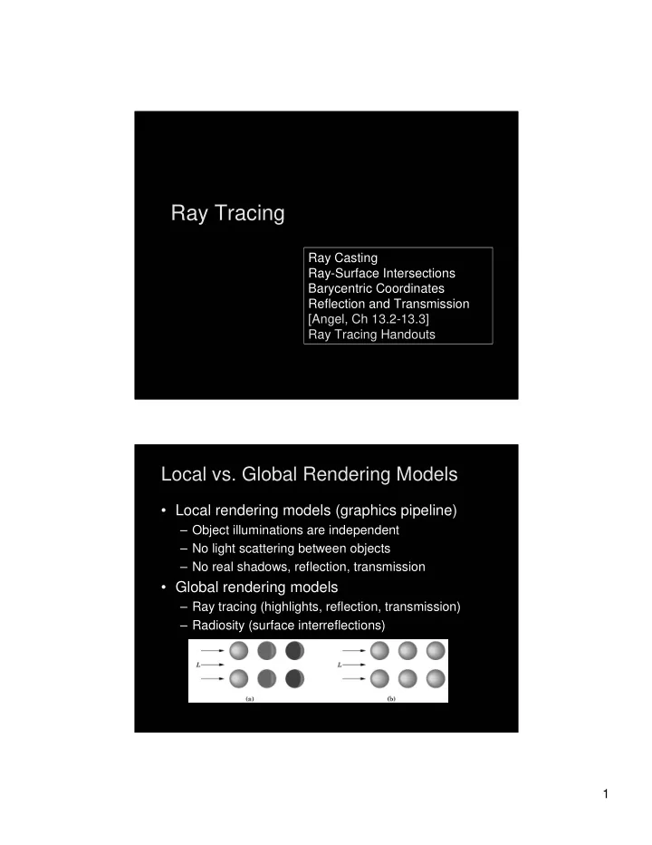
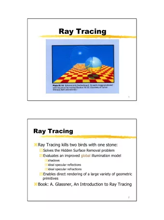
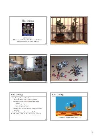
Ray Tracing Ray Tracing Ray Casting Ray Casting Ray-Surface Intersections Ray-Surface Intersections Barycentric Coordinates Barycentric Coordinates Reflection and Transmission Reflection and Transmission [Angel, Ch 13.2-13.3] [Angel, Ch 13.2-13.3] Ray Tracing Handouts Ray Tracing Handouts Local vs. Global Rendering Models Local vs. Global Rendering Models • Local rendering models (graphics pipeline) – Object illuminations are independent – No light scattering between objects – No real shadows, reflection, transmission • Global rendering models – Ray tracing (highlights, reflection, transmission) – Radiosity (surface interreflections) 1

Object Space vs. Image Space Object Space vs. Image Space • Graphics pipeline: for each object, render – Efficient pipeline architecture, on-line – Difficulty: object interactions • Ray tracing: for each pixel, determine color – Pixel-level parallelism, off-line – Difficulty: efficiency, light scattering • Radiosity: for each two surface patches, determine diffuse interreflections – Solving integral equations, off-line – Difficulty: efficiency, reflection Forward Ray Tracing Forward Ray Tracing • Rays as paths of photons in world space • Forward ray tracing: follow photon from light sources to viewer • Problem: many rays will not contribute to image! 2

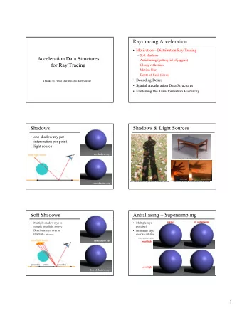
Backward Ray Tracing Backward Ray Tracing • Ray-casting: one ray from center of projection through each pixel in image plane • Illumination 1. Phong (local as before) 2. Shadow rays 3. Specular reflection 4. Specular transmission • (3) and (4) are recursive Shadow Rays Shadow Rays • Determine if light “really” hits surface point • Cast shadow ray from surface point to light • If shadow ray hits opaque object,no contribution • Improved diffuse reflection 3

Reflection Rays Reflection Rays • Calculate specular component of illumination • Compute reflection ray (recall: backward!) • Call ray tracer recursively to determine color • Add contributions • Transmission ray – Analogue for transparent or translucent surface – Use Snell’s laws for refraction • Later: – Optimizations, stopping criteria Ray Casting Ray Casting • Simplest case of ray tracing • Required as first step of recursive ray tracing • Basic ray-casting algorithm – For each pixel (x,y) fire a ray from COP through (x,y) – For each ray & object calculate closest intersection – For closest intersection point p • Calculate surface normal • For each light source, calculate and add contributions • Critical operations – Ray-surface intersections – Illumination calculation 4

Recursive Ray Tracing Recursive Ray Tracing • Calculate specular component – Reflect ray from eye on specular surface – Transmit ray from eye through transparent surface • Determine color of incoming ray by recursion • Trace to fixed depth • Cut off if contribution below threshold Angle of Reflection Angle of Reflection • Recall: incoming angle = outgoing angle • r = 2( l � n ) n – l • For incoming/outgoing ray negate l ! • Compute only for surfaces with actual reflection • Use specular coefficient • Add specular and diffuse components 5

Refraction Refraction • Index of refraction is relative speed of light • Snell’s law – � l = index of refraction for upper material – � t = index of refraction for lower material [U = �� Raytracing Example Raytracing Example www.povray.org 6

Raytracing Example Raytracing Example rayshade gallery Raytracing Example Raytracing Example rayshade gallery 7

Raytracing Example Raytracing Example www.povray.org Raytracing Example Raytracing Example Saito, Saturn Ring 8

Raytracing Example Raytracing Example www.povray.org Raytracing Example Raytracing Example www.povray.org 9

Raytracing Example Raytracing Example rayshade gallery Intersections Intersections 10

Ray-Surface Intersections Ray-Surface Intersections • General implicit surfaces • General parametric surfaces • Specialized analysis for special surfaces – Spheres – Planes – Polygons – Quadrics • Do not decompose objects into triangles! • CSG is also a good possibility Rays and Parametric Surfaces Rays and Parametric Surfaces • Ray in parametric form – Origin p 0 = [x 0 y 0 z 0 1] T – Direction d = [x d y d z d 0] t 2 + y d 2 + z d 2 = 1) – Assume d normalized (x d – Ray p (t) = p 0 + d t for t > 0 • Surface in parametric form – Point q = g(u, v), possible bounds on u, v – Solve p + d t = g(u, v) – Three equations in three unknowns (t, u, v) 11

Rays and Implicit Surfaces Rays and Implicit Surfaces • Ray in parametric form – Origin p 0 = [x 0 y 0 z 0 1] T – Direction d = [x d y d z d 0] t 2 + y d 2 + z d 2 = 1) – Assume d normalized (x d – Ray p (t) = p 0 + d t for t > 0 • Implicit surface – Given by f( q ) = 0 – Consists of all points q such that f( q ) = 0 – Substitute ray equation for q : f( p 0 + d t) = 0 – Solve for t (univariate root finding) – Closed form (if possible) or numerical approximation Ray-Sphere Intersection I Ray-Sphere Intersection I • Common and easy case • Define sphere by – Center c = [x c y c z c 1] T – Radius r – Surface f( q ) = (x – x c ) 2 + (y – y c ) 2 + (z – z c ) 2 – r 2 = 0 • Plug in ray equations for x, y, z: 12

Ray-Sphere Intersection II Ray-Sphere Intersection II • Simplify to where • Solve to obtain t 0 and t 1 Check if t 0 , t 1 > 0 (ray) Return min(t 0 , t 1 ) Ray-Sphere Intersection III Ray-Sphere Intersection III • For lighting, calculate unit normal • Negate if ray originates inside the sphere! 13

Simple Optimizations Simple Optimizations • Factor common subexpressions • Compute only what is necessary – Calculate b 2 – 4c, abort if negative – Compute normal only for closest intersection – Other similar optimizations [Handout] Ray-Polygon Intersection I Ray-Polygon Intersection I • Assume planar polygon 1. Intersect ray with plane containing polygon 2. Check if intersection point is inside polygon • Plane – Implicit form: ax + by + cz + d = 0 Unit normal: n = [a b c 0] T with a 2 + b 2 + c 2 = 1 – • Substitute: • Solve: 14

Ray-Polygon Intersection II Ray-Polygon Intersection II • Substitute t to obtain intersection point in plane • Test if point inside polygon [see Handout] Ray-Quadric Intersection Ray-Quadric Intersection • Quadric f( p ) = f(x, y, z) = 0, where f is polynomial of order 2 • Sphere, ellipsoid, paraboloid, hyperboloid, cone, cylinder • Closed form solution as for sphere • Important case for modelling in ray tracing • Combine with CSG [see Handout] 15

Barycentric Coordinates Barycentric Coordinates Interpolated Shading for Ray Tracing Interpolated Shading for Ray Tracing • Assume we know normals at vertices • How do we compute normal of interior point? • Need linear interpolation between 3 points • Barycentric coordinates • Yields same answer as scan conversion 16

Barycentric Coordinates in 1D Barycentric Coordinates in 1D • Linear interpolation – p (t) = (1 – t) p 1 + t p 2 , 0 � t � 1 – p (t) = � p 1 + � p 2 where � + � = 1 – p is between p 1 and p 2 iff 0 � � , � � 1 • Geometric intuition – Weigh each vertex by ratio of distances from ends p 1 p p 2 � � • � , � are called barycentric coordinates Barycentric Coordinates in 2D Barycentric Coordinates in 2D • Given 3 points instead of 2 p 1 p p 2 p 3 • Define 3 barycentric coordinates, � , � , � • p = � p 1 + � p 2 + � p 3 • p inside triangle iff 0 � � , � , � � 1, � + � + � = 1 • How do we calculate � , � , � given p ? 17

Barycentric Coordinates for Triangle Barycentric Coordinates for Triangle • Coordinates are ratios of triangle areas CC C Area C � � 1 2 1 � � C C C Area � 0 1 2 � C CC Area � � 0 2 C � � � C C C Area � � 0 1 2 � C C C C Area � 2 � � 1 0 1 � � � � � � � C C C Area C � � 0 1 2 0 Computing Triangle Area Computing Triangle Area C • In 3 dimensions – Use cross product B – Parallelogram formula A – Area(ABC) = (1/2)|(B – A) � (C – A)| – Optimization: project, use 2D formula • In 2 dimensions – Area(x-y-proj(ABC)) = (1/2)((b x – a x )(c y – a y ) – (c x – a x ) (b y – a y )) 18

Ray Tracing Preliminary Assessment Ray Tracing Preliminary Assessment • Global illumination method • Image-based • Pros: – Relatively accurate shadows, reflections, refractions • Cons: – Slow (per pixel parallelism, not pipeline parallelism) – Aliasing – Inter-object diffuse reflections Ray Tracing Acceleration Ray Tracing Acceleration • Faster intersections – Faster ray-object intersections • Object bounding volume • Efficient intersectors – Fewer ray-object intersections • Hierarchical bounding volumes (boxes, spheres) • Spatial data structures • Directional techniques • Fewer rays – Adaptive tree-depth control – Stochastic sampling • Generalized rays (beams, cones) 19

20