Rational function approximation Rational function of degree N = n + m - PowerPoint PPT Presentation

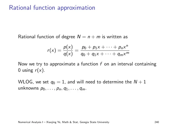
Rational function approximation Rational function of degree N = n + m is written as q ( x ) = p 0 + p 1 x + · · · + p n x n r ( x ) = p ( x ) q 0 + q 1 x + · · · + q m x m Now we try to approximate a function f on an interval containing 0 using r ( x ). WLOG, we set q 0 = 1, and will need to determine the N + 1 unknowns p 0 , . . . , p n , q 1 , . . . , q m . Numerical Analysis I – Xiaojing Ye, Math & Stat, Georgia State University 240

Pad´ e approximation The idea of Pad´ e approximation is to find r ( x ) such that f ( k ) (0) = r ( k ) (0) , k = 0 , 1 , . . . , N This is an extension of Taylor series but in the rational form. Denote the Maclaurin series expansion f ( x ) = � ∞ i =0 a i x i . Then i =0 q i x i − � n � ∞ i =0 a i x i � m i =0 p i x i f ( x ) − r ( x ) = q ( x ) If we want f ( k ) (0) − r ( k ) (0) = 0 for k = 0 , . . . , N , we need the numerator to have 0 as a root of multiplicity N + 1. Numerical Analysis I – Xiaojing Ye, Math & Stat, Georgia State University 241

Pad´ e approximation This turns out to be equivalent to k � a i q k − i = p k , k = 0 , 1 , . . . , N i =0 for convenience we used convention p n +1 = · · · = p N = 0 and q m +1 = · · · = q N = 0. From these N + 1 equations, we can determine the N + 1 unknowns: p 0 , p 1 , . . . , p n , q 1 , . . . , q m Numerical Analysis I – Xiaojing Ye, Math & Stat, Georgia State University 242

Pad´ e approximation Example e approximation to e − x of degree 5 with n = 3 and Find the Pad´ m = 2. Solution. We first write the Maclaurin series of e − x as ∞ ( − 1) i e − x = 1 − x + 1 2 x 2 − 1 6 x 3 + 1 24 x 4 + · · · = � x i i ! i =0 Then for r ( x ) = p 0 + p 1 x + p 2 x 2 + p 3 x 3 , we need 1+ q 1 x + q 2 x 2 1 − x + 1 2 x 2 − 1 � 6 x 3 + · · · � (1+ q 1 x + q 2 x 2 ) − p 0 + p 1 x + p 2 x 2 + p 3 x 3 to have 0 coefficients for terms 1 , x , . . . , x 5 . Numerical Analysis I – Xiaojing Ye, Math & Stat, Georgia State University 243

Pad´ e approximation Solution. (cont.) By solving this, we get p 0 , p 1 , p 2 , q 1 , q 2 and hence 20 x 2 − 1 r ( x ) = 1 − 3 5 x + 3 60 x 3 1 + 2 5 x + 1 20 x 2 e − x | e − x − P 5 ( x ) | | e − x − r ( x ) | x P 5 ( x ) r ( x ) 8.64 × 10 − 8 7.55 × 10 − 9 0.2 0.81873075 0.81873067 0.81873075 5.38 × 10 − 6 4.11 × 10 − 7 0.4 0.67032005 0.67031467 0.67031963 5.96 × 10 − 5 4.00 × 10 − 6 0.6 0.54881164 0.54875200 0.54880763 3.26 × 10 − 4 1.93 × 10 − 5 0.8 0.44932896 0.44900267 0.44930966 1.21 × 10 − 3 6.33 × 10 − 5 1.0 0.36787944 0.36666667 0.36781609 where P 5 ( x ) is Maclaurin polynomial of degree 5 for comparison. Numerical Analysis I – Xiaojing Ye, Math & Stat, Georgia State University 244

Chebyshev rational function approximation To obtain more uniformly accurate approximation, we can use Chebyshev polynomials T k ( x ) in Pad´ e approximation framework. For N = n + m , we use � n k =0 p k T k ( x ) r ( x ) = � m k =0 q k T k ( x ) where q 0 = 1. Also write f ( x ) using Chebyshev polynomials as ∞ � f ( x ) = a k T k ( x ) k =0 Numerical Analysis I – Xiaojing Ye, Math & Stat, Georgia State University 245

Chebyshev rational function approximation Now we have � ∞ k =0 a k T k ( x ) � m k =0 q k T k ( x ) − � n k =0 p k T k ( x ) f ( x ) − r ( x ) = � m k =0 q k T k ( x ) We again seek for p 0 , . . . , p n , q 1 , . . . , q m such that coefficients of 1 , x , . . . , x N are 0. To that end, the computations can be simplified due to T i ( x ) T j ( x ) = 1 � � T i + j ( x ) + T | i − j | ( x ) 2 Also note that we also need to compute Chebyshev series coefficients a k first. Numerical Analysis I – Xiaojing Ye, Math & Stat, Georgia State University 246

Chebyshev rational function approximation Example Approximate e − x using the Chebyshev rational approximation of degree n = 3 and m = 2. The result is r T ( x ). e − x | e − x − r ( x ) | | e − x − r T ( x ) | x r ( x ) r T ( x ) 7.55 × 10 − 9 5.66 × 10 − 6 0.2 0.81873075 0.81873075 0.81872510 4.11 × 10 − 7 6.95 × 10 − 6 0.4 0.67032005 0.67031963 0.67031310 4.00 × 10 − 6 1.28 × 10 − 6 0.6 0.54881164 0.54880763 0.54881292 1.93 × 10 − 5 9.13 × 10 − 6 0.8 0.44932896 0.44930966 0.44933809 6.33 × 10 − 5 7.89 × 10 − 6 1.0 0.36787944 0.36781609 0.36787155 where r ( x ) is the standard Pad´ e approximation shown earlier. Numerical Analysis I – Xiaojing Ye, Math & Stat, Georgia State University 247

Trigonometric polynomial approximation Recall the Fourier series uses a set of 2 n orthogonal functions with respect to weight w ≡ 1 on [ − π, π ]: φ 0 ( x ) = 1 2 φ k ( x ) = cos kx , k = 1 , 2 , . . . , n φ n + k ( x ) = sin kx , k = 1 , 2 , . . . , n − 1 We denote the set of linear combinations of φ 0 , φ 1 , . . . , φ 2 n − 1 by T n , called the set of trigonometric polynomials of degree ≤ n . Numerical Analysis I – Xiaojing Ye, Math & Stat, Georgia State University 248

Trigonometric polynomial approximation For a function f ∈ C [ − π, π ], we want to find S n ∈ T n of form n − 1 S n ( x ) = a 0 � 2 + a n cos nx + ( a k cos kx + b k sin kx ) k =1 to minimize the least squares error � π | f ( x ) − S n ( x ) | 2 d x E ( a 0 , . . . , a n , b 1 , . . . , b n − 1 ) = − π Due to orthogonality of Fourier series φ 0 , . . . , φ 2 n − 1 , we get � π � π a k = 1 b k = 1 f ( x ) cos kx d x , f ( x ) sin kx d x π π − π − π Numerical Analysis I – Xiaojing Ye, Math & Stat, Georgia State University 249

Trigonometric polynomial approximation Example Approximate f ( x ) = | x | for x ∈ [ − π, π ] using trigonometric polynomial from T n . � π Solution. It is easy to check that a 0 = 1 − π | x | d x = π and π � π a k = 1 2 π k 2 (( − 1) k − 1) , | x | cos kx d x = k = 1 , 2 , . . . , n π − π � π b k = 1 | x | sin kx d x = 0 , k = 1 , 2 , . . . , n − 1 π − π Therefore ( − 1) k − 1 n 2 + 2 S n ( x ) = π � cos kx k 2 π k =1 Numerical Analysis I – Xiaojing Ye, Math & Stat, Georgia State University 250

Trigonometric polynomial approximation S n ( x ) for the first few n are shown below: y y � � x � π y � S 3 ( x ) � � 4 4 π cos x � cos 3 x 2 9 π π y � S 1 ( x ) � S 2 ( x ) � � 4 π cos x 2 π π y � S 0 ( x ) � π 2 2 x π π � π π � 2 2 Numerical Analysis I – Xiaojing Ye, Math & Stat, Georgia State University 251

Discrete trigonometric approximation If we have 2 m paired data points { ( x j , y j ) } 2 m − 1 where x j are j =0 equally spaced on [ − π, π ], i.e., � j � x j = − π + j = 0 , 1 , . . . , 2 m − 1 π, m Then we can also seek for S n ∈ T n such that the discrete least square error below is minimized: 2 m − 1 � ( y j − S n ( x j )) 2 E ( a 0 , . . . , a n , b 1 , . . . , b n − 1 ) = j =0 Numerical Analysis I – Xiaojing Ye, Math & Stat, Georgia State University 252

Discrete trigonometric approximation Theorem Define 2 m − 1 2 m − 1 a k = 1 b k = 1 � � y j cos kx j , y j sin kx j m m j =0 j =0 Then the trigonometric S n ∈ T n defined by n − 1 S n ( x ) = a 0 � 2 + a n cos nx + ( a k cos kx + b k sin kx ) k =1 minimizes the discrete least squares error 2 m − 1 � ( y j − S n ( x j )) 2 E ( a 0 , . . . , a n , b 1 , . . . , b n − 1 ) = j =0 Numerical Analysis I – Xiaojing Ye, Math & Stat, Georgia State University 253

Fast Fourier transforms The fast Fourier transform (FFT) employs the Euler formula e z i = cos z + i sin z for all z ∈ R and i = √− 1, and compute the discrete Fourier transform of data to get 2 m − 1 2 m − 1 1 y j e k π i / m k = 0 , . . . , 2 m − 1 � � c k e kx i , where c k = m k =0 j =0 Then one can recover a k , b k ∈ R from a k + i b k = ( − 1) k c k ∈ C m Numerical Analysis I – Xiaojing Ye, Math & Stat, Georgia State University 254

Fast Fourier transforms The discrete trigonometric approximation for 2 m data points requires a total of (2 m ) 2 multiplications, not scalable for large m . The cost of FFT is only 3 m + m log 2 m = O ( m log 2 m ) For example, if m = 1024, then (2 m ) 2 ≈ 4 . 2 × 10 6 and 3 m + m log 2 m ≈ 1 . 3 × 10 4 . The larger m is, the more benefit FFT gains. Numerical Analysis I – Xiaojing Ye, Math & Stat, Georgia State University 255