Zeros and poles of Pad e approximants to the symmetric Zeta - PDF document

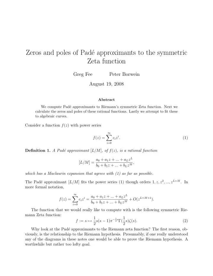
Zeros and poles of Pad´ e approximants to the symmetric Zeta function Greg Fee Peter Borwein August 19, 2008 Abstract We compute Pad´ e approximants to Riemann’s symmetric Zeta function. Next we calculate the zeros and poles of these rational functions. Lastly we attempt to fit these to algebraic curves. Consider a function f ( z ) with power series ∞ � c i z i . f ( z ) = (1) i =0 Definition 1. A Pad´ e approximant [ L/M ] , of f ( z ) , is a rational function [ L/M ] = a 0 + a 1 z + ... + a L z L b 0 + b 1 z + ... + b L z M , which has a Maclaurin expansion that agrees with (1) as far as possible. The Pad´ e approximant [ L/M ] fits the power series (1) though orders 1 , z, z 2 , ..., z L + M . In more formal notation, ∞ c i z i = a 0 + a 1 z + ... + a L z L � b 0 + b 1 z + ... + b L z M + O ( z L + M +1 ) . f ( z ) = i =0 The function that we would really like to compute with is the following symmetric Rie- mann Zeta function: f := s �→ 1 2 s Γ(1 2 s ( s − 1) π − 1 2 s ) ζ ( s ) . (2) Why look at the Pad´ e approximants to the Riemann zeta function? The first reason, ob- viously, is the relationship to the Riemann hypothesis. Presumably, if one really understood any of the diagrams in these notes one would be able to prove the Riemann hypothesis. A worthwhile but rather too lofty goal.

2 But even assuming the Riemann hypothesis the particular behavior of the approximations is not obvious. Clearly there are limit curves both of the zeros and the poles. One goal is to figure out what these probably are. It is harder than it looks to generate these pictures. Standard symbolic packages fail. So another part of the story is to describe the necessary computations. There is a lovely body of theory due originally to Szeg¨ o that describes the zeros of the partial sums up the power series expansion of the exponential function. This extends to the zeros and poles of the Pad´ e approximants to the exponential function and a few related functions. In order to get limit curves one scales the zeros and poles by dividing by the degree. The analysis is possible because there are explicit integral representations of the numerators and denominators. There are no useful explicit representations known for the Pad´ e approximants to the zeta function. Or even for the Taylor series. And indeed the principal problem in generating the approximations numerically is to derive large Taylor expansions. This is the principal story that we want to tell in this paper. And to describe the computational difficulties that it involves. List of Figures Order 2 6 + 1: Taylor series. 1 . . . . . . . . . . . . . . . . . . . . . . . . . . . 3 Order 2 7 + 1: Taylor series. 2 . . . . . . . . . . . . . . . . . . . . . . . . . . . 3 Order 2 8 + 1: Taylor series. 3 . . . . . . . . . . . . . . . . . . . . . . . . . . . 4 Order 2 9 + 1: Taylor series. 4 . . . . . . . . . . . . . . . . . . . . . . . . . . . 4 Order 2 10 + 1: Taylor series. . . . . . . . . . . . . . . . . . . . . . . . . . . . 5 5 6 Fit curves: Taylor series. . . . . . . . . . . . . . . . . . . . . . . . . . . . . . 6 Order 2 6 + 1: all Pad´ 7 e approximants. . . . . . . . . . . . . . . . . . . . . . . 7 Order 2 7 + 1: all Pad´ 8 e approximants. . . . . . . . . . . . . . . . . . . . . . . 7 Order 2 4 + 1: diagonal Pad´ 9 e approximant. . . . . . . . . . . . . . . . . . . . 8 Order 2 5 + 1: diagonal Pad´ 10 e approximant. . . . . . . . . . . . . . . . . . . . 8 Order 2 6 + 1: diagonal Pad´ 11 e approximant. . . . . . . . . . . . . . . . . . . . 9 Order 2 7 + 1: diagonal Pad´ 12 e approximant. . . . . . . . . . . . . . . . . . . . 10 Order 2 7 + 1: diagonal Pad´ 13 e approximant expanded about various points. . . 11 Order 2 8 + 1: diagonal Pad´ 14 e approximant. . . . . . . . . . . . . . . . . . . . 12 Order 2 9 + 1: diagonal Pad´ 15 e approximant. . . . . . . . . . . . . . . . . . . . 13 Order 2 10 + 1: diagonal Pad´ 16 e approximant. . . . . . . . . . . . . . . . . . . . 14

Taylor Series. 3 1 Taylor Series (a) All zeros. (b) Quadrant I of Figure (a) with degree 2 curve fit to extraneous zeros. Figure 1: Zeros of the truncated Taylor series of order 2 6 +1 of the symmetric Zeta function. (a) All zeros. (b) Quadrant I of Figure (a) with degree 2 curve fit to extraneous zeros. Figure 2: Zeros of the truncated Taylor series of order 2 7 +1 of the symmetric Zeta function.

Taylor Series. 4 (a) All zeros. (b) Quadrant I of Figure (a) with degree 2 curve fit to extraneous zeros. Figure 3: Zeros of the truncated Taylor series of order 2 8 +1 of the symmetric Zeta function. (a) All zeros. (b) Quadrant I of Figure (a) with degree 2 curve fit to extraneous zeros. Figure 4: Zeros of the truncated Taylor series of order 2 9 +1 of the symmetric Zeta function.

Taylor Series. 5 (a) All zeros. (b) Quadrant I of Figure (a) with degree 2 curve fit to extraneous zeros. Figure 5: Zeros of the truncated Taylor series of order 2 10 +1 of the symmetric Zeta function.

Taylor Series. 6 (a) Curve from Figure 1(b): (b) Curve from Figure 2(b): 0 . 998759 + 0 . 010069 x − 0 . 048769 y − 0 . 999563 + 0 . 006174 x − 0 . 028906 y − 0 . 000351 x 2 − 0 . 000115 xy +0 . 000365 y 2 . 0 . 000147 x 2 − 0 . 000035 xy +0 . 000010 y 2 . (c) Curve from Figure 3(b): (d) Curve from Figure 4(b): 0 . 999844 + 0 . 003601 x − 0 . 017305 y − 0 . 999949 + 0 . 002524 x − 0 . 009778 y − 0 . 000055 x 2 − 0 . 000009 xy +0 . 000032 y 2 . 0 . 000021 x 2 − 0 . 000005 xy +0 . 000007 y 2 . (e) Curve from Figure 5(b): 0 . 99998397233832516156127808097689+ 0 . 0017114866390274882214362533125239 x − 0 . 0053968338455743015329285156850858 y − 0 . 0000076913868171049289130164708154098 x 2 − 0 . 0000021399957002464736373025075642063 xy + 0 . 00000080896194920156322933685037036162 y 2 . Figure 6: Curves that fit extraneous zeros in Figures 1–5.

All Pad´ e approximants together. 7 2 All Pad´ e approximants together (a) Poles. (b) Zeros. Figure 7: Zeros and poles of all Pade approximants [L/M] for L+M = 64 (a) Poles. (b) Zeros. Figure 8: Zeros of all Pade approximants [L/M] for L+M = 128

Order 2 4 + 1 . 8 Order 2 4 + 1 3 Figure 9: Red zeros and blue poles of the [8/8] Pad´ e approximant about x = 1 / 2 to the symmetric Zeta function. Order 2 5 + 1 4 Figure 10: Red zeros and blue poles of the [16/16] Pad´ e approximant about x = 1 / 2 to the symmetric Zeta function.

Order 2 6 + 1 . 9 Order 2 6 + 1 5 (a) Zeros and poles. (b) Fit degree 2 curve to the poles in quadrants I and IV. (c) Fit degree 2 curve to the zeros in quadrants I (d) Quadrant I of Figure (a) with curves fit to zeros and IV. and poles. Figure 11: Various views of the red zeros and blue poles of the [32/32] Pad´ e approximant about x = 1 / 2 to the symmetric Zeta function.

Order 2 7 + 1 . 10 Order 2 7 + 1 6 (a) Zeros and poles. (b) Fit degree 2 curve to the poles in quadrants I and IV. (c) Fit degree 2 curve to the zeros in quadrants I (d) Figures (b) and (c) together. and IV. Figure 12: Various views of the red zeros and blue poles of the [64/64] Pad´ e approximant about x = 1 / 2 to the symmetric Zeta function.

Order 2 7 + 1 . 11 (a) Expand about x = 0. (b) Quadrant I of Figure (a). (c) Expand about x = 1 / 2. (d) Quadrant I of Figure (c). (e) Expand about x = 1. (f) Quadrant I of Figure (e). Figure 13: Views of the [64/64] Pad´ e approximant expanded about various x values

Order 2 8 + 1 . 12 Order 2 8 + 1 7 (a) Zeros and poles. (b) Quadrant I of Figure (a). (c) Fit degree 2 curves to Figure (b). Figure 14: Various views of the red zeros and blue poles of the [128/128] Pad´ e approximant about x = 1 / 2 to the symmetric Zeta function.

Order 2 9 + 1 . 13 Order 2 9 + 1 8 (a) Zeros and poles. (b) Quadrant I of Figure (a). (c) Fit degree 2 curves to Figure (b). Figure 15: Various views of the red zeros and blue poles of the [256/256] Pad´ e approximant about x = 1 / 2 to the symmetric Zeta function.

Order 2 10 + 1 . 14 Order 2 10 + 1 9 (a) Zeros and poles. (b) Quadrant I of Figure (a). (c) Fit degree 2 curves to Figure (b). Figure 16: Various views of the red zeros and blue poles of the [512/512] Pad´ e approximant about x = 1 / 2 to the symmetric Zeta function.