Randomized algorithms Guessing cards Three examples: - PowerPoint PPT Presentation

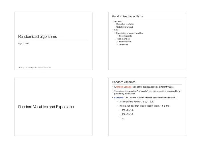
Randomized algorithms • Last week • Contention resolution • Global minimum cut • Today • Expectation of random variables Randomized algorithms • Guessing cards • Three examples: • Median/Select. Inge Li Gørtz • Quick-sort Thank you to Kevin Wayne for inspiration to slides Random variables • A random variable is an entity that can assume di ff erent values. • The values are selected “randomly”; i.e., the process is governed by a probability distribution. • Examples: Let X be the random variable “number shown by dice”. • X can take the values 1, 2, 3, 4, 5, 6. Random Variables and Expectation • If it is a fair dice then the probability that X = 1 is 1/6: • P[X=1] =1/6. • P[X=2] =1/6. • …

Expected values Waiting for a first succes • Let X be a random variable with values in {x 1 ,…x n }, where x i are • Coin flips. Coin is heads with probability and tails with probability . How p 1 − p numbers. many independent flips X until first heads? • Probability of ? (first succes is in round ) X = j j • The expected value (expectation) of X is defined as Pr[ X = j ] = (1 − p ) j − 1 ⋅ p n ∑ • Expected value of : X E [ X ] = x j ⋅ Pr[ X = x j ] ∞ ∑ j =1 E [ X ] = j ⋅ Pr[ X = j ] j =1 • The expectation is the theoretical average. ∞ ∑ j ⋅ (1 − p ) j − 1 ⋅ p = • Example: j =1 ∞ p • X = random variable “number shown by dice” ∑ j ⋅ (1 − p ) j = ∞ x ∑ k ⋅ x k = 1 − p (1 − x ) 2 6 j =1 j ⋅ Pr[ X = j ] = (1 + 2 + 3 + 4 + 5 + 6) ⋅ 1 k =0 ∑ E [ X ] = 6 = 3.5 1 − p ⋅ 1 − p p = 1 = for . | x | < 1 p 2 p j =1 Properties of expectation Guessing cards • If we repeatedly perform independent trials of an experiment, each of • Game. Shu ffl e a deck of cards; turn them over one at a time; try to guess each n card. which succeeds with probability , then the expected number of p > 0 • Memoryless guessing. Can't remember what's been turned over already. Guess a trials we need to perform until the first succes is . 1/ p card from full deck uniformly at random. • Claim. The expected number of correct guesses is 1 . • If is a 0/1 random variable, . X E [ X ] = Pr[ X = 1] i th if guess correct and zero otherwise. • X i = 1 the correct number of guesses . • X = = X 1 + … + X n • Linearity of expectation: For two random variables X and Y we have • . E [ X i ] = Pr[ X i = 1] = 1/ n E [ X + Y ] = E [ X ] + E [ Y ] • E [ X ] = E [ X 1 + ⋯ + X n ] = E [ X 1 ] + ⋯ + E [ X n ] = 1/ n + ⋯ + 1/ n = 1.

Guessing cards Coupon collector • Game. Shu ffl e a deck of n cards; turn them over one at a time; try to guess each • Coupon collector. Each box of cereal contains a coupon. There are di ff erent types n card. of coupons. Assuming all boxes are equally likely to contain each coupon, how many boxes before you have at least 1 coupon of each type? • Guessing with memory. Guess a card uniformly at random from cards not yet seen. • Claim. The expected number of steps is . • Claim. The expected number of correct guesses is . Θ ( n log n ) Θ (log n ) • Phase = time between and distinct coupons. if i th guess correct and zero otherwise. j j j + 1 • X i = 1 = number of steps you spend in phase . • X j j • the correct number of guesses . X = = X 1 + … + X n . • = number of steps in total = X 0 + X 1 + ⋯ + X n − 1 . • E [ X i ] = Pr[ X i = 1] = 1/( n − i − 1) X . • E [ X ] = E [ X 1 ] + ⋯ + E [ X n ] = 1/ n + ⋯ + 1/2 + 1/1 = H n . • E [ X j ] = n /( n − j ) • The expected number of steps: ln n < H ( n ) < ln n + 1 n − 1 n − 1 n − 1 n ∑ ∑ ∑ ∑ . E [ X ] = E [ X j ] = E [ X j ] = n /( n − j ) = n ⋅ 1/ i = n ⋅ H n j =0 j =0 j =0 i =1 Select • Given n numbers S = {a 1 , a 2 , …, a n }. • Median: number that is in the middle position if in sorted order. • Select(S,k): Return the kth smallest number in S. • Min(S) = Select(S,1), Max(S)= Select(S,n), Median = Select(S,n/2). • Assume the numbers are distinct. Median/Select Select(S, k) { Choose a pivot s ∈ S uniformly at random. For each element e in S if e < s put e in S’ if e > s put e in S’’ if |S’| = k-1 then return s if |S’| ≥ k then call Select(S’, k) if |S’| < k then call Select(S’’, k - |S’| - 1) }

Select Select n (3 / 4) j +1 • Phase j: Size of set at most and at least . n (3 / 4) j Select(S, k) { • Central element: at least a quarter of the elements in the current call are smaller and Choose a pivot s ∈ S uniformly at random. at least a quarter are larger. For each element e in S if e < s put e in S’ • At least half the elements are central. if e > s put e in S’’ • Pivot central => size of set shrinks with by at least a factor 3/4 => current phase if |S’| = k-1 then return s ends. if |S’| ≥ k then call Select(S’, k) • Pr[s is central] = 1/2. if |S’| < k then call Select(S’’, k - |S’| - 1) • Expected number of iterations before a central pivot is found = 2 => } expected number of iterations in phase j at most 2. T ( n ) = cn + c ( n − 1) + c ( n − 2) + · · · = Θ ( n 2 ) . • Worst case running time: • X: random variable equal to number of steps taken by algorithm. • If there is at least an fraction of elements both larger and smaller than s: ε • X j : expected number of steps in phase j. cn + (1 − ε ) cn + (1 − ε ) 2 cn + · · · T ( n ) = • X = X 1 + X 2 + .… 1 + (1 − ε ) + (1 − ε ) 2 + · · · = � � cn • Number of steps in one iteration in phase j is at most . cn (3 / 4) j cn/ ε . ≤ E [ X j ] = 2 cn (3/4) j . • 2 cn ( j j • Limit number of bad pivots. E [ X ] = ∑ E [ X j ] ≤ ∑ 4 ) j ( 4 ) 3 3 = 2 cn ∑ • Expected running time: ≤ 8 cn • Intuition: A fairly large fraction of elements are “well-centered” => random pivot j j likely to be good. Quicksort • Given n numbers S = {a 1 , a 2 , …, a n } return the sorted list. • Assume the numbers are distinct. Quicksort(A,p,r) { if |S| ≤ 1 return S Quicksort else Choose a pivot s ∈ S uniformly at random. For each element e in S if e < s put e in S’ if e > s put e in S’’ L = Quicksort(S’) R = Quicksort(S’’) Return the sorted list L ◦ s ◦ R. }

Quicksort: Analysis Quicksort: Analysis • Worst case Quicksort requires Ω (n 2 ) comparisons: if pivot is the smallest element in • Expected number of comparisons: the list in each recursive call. n − 1 n n − 1 n ∑ ∑ ∑ ∑ E [ X ] = E [ X ij ] = E [ X ij ] • If pivot always is the median then T(n) = O(n log n). • for i < j: random variable i =1 j = i +1 i =1 j = i +1 • Since only takes values 0 and 1: X ij E [ X ij ] = Pr[ X ij = 1] ( 1 if a i and a j compared by algorithm X ij = and compared i ff or is the first pivot chosen from . • a i a j a i a j Z ij = { a i , …, a j } 0 otherwise • Pivot chosen independently uniformly at random all elements from equally ⇒ Z ij • X total number of comparisons: likely to be chosen as first pivot from this set. n − 1 n X X • We have Pr[ X ij = 1] = 2/( j − i + 1) X = X ij i =1 j = i +1 • Thus n − 1 n n − 1 n n − 1 n 2 • Expected number of comparisons: ∑ ∑ ∑ ∑ ∑ ∑ E [ X ] = E [ X ij ] = Pr[ X ij = 1] = j − i + 1 n − 1 n n − 1 n i =1 j = i +1 i =1 j = i +1 i =1 j = i +1 ∑ ∑ ∑ ∑ E [ X ] = E [ X ij ] = E [ X ij ] n − 1 n − i +1 n − 1 n n − 1 2 2 i =1 j = i +1 i =1 j = i +1 ∑ ∑ ∑ ∑ ∑ = < = O (log n ) = O ( n log n ) k k i =1 k =2 i =1 k =1 i =1