Random Walk Based Algorithms for Complex Network Analysis - PowerPoint PPT Presentation
Random Walk Based Algorithms for Complex Network Analysis Konstantin Avrachenkov Inria Sophia Antipolis Rescom 2014, 12-16 May, Furiani, Corse Complex networks Main features of complex networks: Sparse topology; Heavy-tail degree
Random Walk Based Algorithms for Complex Network Analysis Konstantin Avrachenkov Inria Sophia Antipolis Rescom 2014, 12-16 May, Furiani, Corse
Complex networks Main features of complex networks: ◮ Sparse topology; ◮ Heavy-tail degree distribution; ◮ Small average distance; ◮ Many triangles.
Complex networks Many complex networks are very large. For instance, ◮ The static part of the web graph has more than 10 billion pages. With an average number of 38 hyper-links per page, the total number of hyper-links is 380 billion. ◮ Twitter has more than 500 million users. On average a user follows about 100 other users. Thus, the number of ”following”-type social relations is about 50 billion.
Complex network analysis Often the topology of a complex network is not known or/and constantly changing. And crawling networks is often subject to a limit on the number of requests per minute. For instance, a standard Twitter account can make no more than one request per minute. With this rate, we would crawl the entire Twitter social network in 950 years...
Complex network analysis Thus, for the analysis of complex networks, it is just essential to use methods with linear or even sub-linear complexity.
Complex network analysis In this tutorial we answer the following questions: ◮ How to estimate quickly the size of a large network? ◮ How to count the number of network motifs? ◮ How to detect quickly most central nodes? ◮ How to partition network in clusters/communities? And we answer these questions by random walk based methods with low complexity.
How to estimate quickly the number of nodes? Suppose that we can only crawl the network. And we would like to estimate quickly the total number of nodes in the network. The first element of our method is the inverse birthday paradox.
How to estimate quickly the number of nodes? In a class of 23 students, the probability of having at least one pair of students with the same birthday is more than 50%! A closely related the inverse birthday paradox says: If we sample repeatedly with replacement, independently and uniformly, from a population of size n , the number of trials √ required for the first repetition has expectation 2 n and variance Θ( √ n ).
How to estimate quickly the number of nodes? Let L be the number of node samples until a repetition occurs. Then, an obvious estimator of the network size is just n = L 2 ˆ 2 . Since the variance is quite high, we need to perform and average several experiments. Theorem Denote by k the number of samples and let n k = 1 / k � k i =1 L 2 ˆ i / 2 . Then, the relative error | ˆ n k − n | / n is less than ε with high probability if we take Θ(1 /ε 2 ) samples.
How to estimate quickly the number of nodes? In many complex networks, generating samples from the uniform distribution is costly or even infeasible. To obtain a sample, which is very close to the uniformly random, we can use either discrete-time or continuous-time random walks.
How to estimate quickly the number of nodes? Let us first consider the discrete-time random walk.
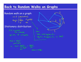
How to estimate quickly the number of nodes? Denote by d i the degree of node i . Then, the stationary distribution of the random walk is given by π i = P { S t = i } = d i 2 m , where m is the number of links. We can unbias the RW sampling by retaining a sample with probability 1 / d i .
How to estimate quickly the number of nodes? Alternatively, we can use a continuous time random walk also choosing uniformly from the list of neighbours and waiting an exponentially distributed time with the mean duration of 1 / d i . In such a case, the stationary distribution is described by the differential equation π ( t ) = π ( t )( A − D ) , ˙ where D = diag { d i } and A is the adjacency matrix � 1 , if ( i , j ) ∈ E , A ij = 0 , otherwise.
How to estimate quickly the number of nodes? For two distributions p and q , let d ( p , q ) denotes the total variation distance: n d ( p , q ) = 1 � | p i − q i | . 2 i =1 The next interpretation is useful: A random sample from distribution p coincides with a random sample from distribution q with probability 1 − d ( p , q ).
How to estimate quickly the number of nodes? Theorem Let λ 2 = min { λ : ( D − A ) x = λ x & λ > 0 } and let π i ( t ) be the distribution of the continuous-time random walk when the process starts at node i. Then, we have 1 e − λ 2 t , d ( π i ( t ) , π ) ≤ 2 √ π i where π is the stationary distribution. In our case, π i = 1 / n . Next, taking t = 3 / 2 log( n ) /λ 2 we obtain d ( π i ( t ) , π ) ≤ 1 2 n .
How to estimate quickly the number of nodes? Thus, we can conclude that the complexity of the continuous-time random walk method on expander-type networks is O ( √ n log( n )), which is sub-linear complexity.
How to estimate quickly the number of links? To estimate the number of edges, we take a different point of view on the random walk. Consider the first return time to node i T + = min { t > 0 : S t = i & S 0 = i } . i The expected value of the first return time is given by i ] = 1 = 2 m E [ T + . π i d i
How to estimate quickly the number of links? Let R k = � k j =1 T k be the time of the k -th return to node i . Then, we can use the following estimator for the number of links m = R k d i ˆ 2 k . To estimate the required complexity, we need to have an idea about the variance of T + i . We can use the following formula i ]) 2 = 2 Z ii + π i − 1 Var [ T + i ] = E [( T + i ) 2 ] − ( E [ T + π 2 π 2 i i with ∞ � Z ii = ( P { S t = i | S 0 = i } − π i ) . t =0
How to estimate quickly the number of links? Next, we note that ∞ ∞ � � Z ii = ( P { S t = i | S 0 = i }− π i ) ≤ | P { S t = i | S 0 = i }− π i | t =0 t =0 and using | P { S t = i | S 0 = i } − π i | ≤ ˜ λ t 2 , we obtain 1 Z ii ≤ , 1 − ˜ λ 2 and hence, 2 Var [ T + i ] � (1 − ˜ λ 2 ) π 2 i or, in our context, 8 m 2 Var [ T + i ] � . (1 − ˜ λ 2 ) d 2 i
Twitter as example
Twitter as example Assuming that a rough estimation of the number of users is 500 · 10 6 and the average number of followers per user is 10, the expected return time from the nodes like “Katy Perry” or “Justin Bieber” is about 2 · 10 · 500 · 10 6 / 50 · 10 6 = 200. To obtain a decent error ( ≤ 5%), we need about 1000 samples, and hence in total about 200000 operations. This is orders of magnitude less than the size of the Twitter follower graph!
How to estimate quickly the number of triangles? To evaluate the degree of clustering in a network, we need to estimate the number of triangle. Towards this goal, we consider a random walk on weighted network where for each link ( i , j ) we assign a weight 1 + t ( i , j ), with t ( i , j ) being the number of triangles containing ( i , j ). The stationary distribution of the random walk on such weighted network is given by d i + � j ∈ N ( i ) t ( i , j ) π i = . 2 m + 6 t ( G )
How to estimate quickly the number of triangles? Thus, if R k = � k j =1 T k is the time of the k -th return to node i , we can use the following estimator � � ( d i + � j ∈ N ( i ) t ( i , j )) R k − m ˆ t ( G ) = max 0 , , 6 k 3 where m is the number of links which we already know how to estimate. Example of the Web graph with 855802 nodes, 5066842 links and 31356298 triangles: Starting from the node with 53371 triangles, the expected return time is 1753. For a good accuracy it was needed to make about 100 returns.
Quick detection of top-k largest degree nodes What if we would like to find quickly in a network top-k nodes with largest degrees? Some applications: ◮ Routing via large degree nodes ◮ Finding influential users in OSN ◮ Proxy for various centrality measures ◮ Node clustering and classification ◮ Epidemic processes on networks
Top-k largest degree nodes Even IF the adjacency list of the network is known... the top-k list of nodes can be found by the HeapSort with complexity O ( n + klog ( n )), where n is the total number of nodes. Even this modest complexity can be quite demanding for large networks (i.e., 950 years for Twitter graph).
Random walk approach Let us again try a random walk approach. We actually recommend the random walk with jumps with the following transition probabilities: � α/ n +1 d i + α , if i has a link to j , p ij = (1) α/ n d i + α , if i does not have a link to j , where d i is the degree of node i and α is a parameter.
Random walk approach This modification can again be viewed as a random walk on weighted graph. Since the weight of link is 1 + α/ n , the stationary distribution of the random walk is given by a simple formula d i + α π i ( α ) = ∀ i ∈ V . (2) 2 | E | + n α
Random walk approach Example: If we run a random walk on the web graph of the UK domain (about 18 500 000 nodes), the random walk spends on average only about 5 800 steps to detect the largest degree node. Three order of magnitude faster than HeapSort!
Recommend
More recommend
Explore More Topics
Stay informed with curated content and fresh updates.


