Random-Variate Generation Banks, Carson, Nelson & Nicol - PowerPoint PPT Presentation
Chapter 8 Random-Variate Generation Banks, Carson, Nelson & Nicol Discrete-Event System Simulation Purpose & Overview Develop understanding of generating samples from a specified distribution as input to a simulation model.
Chapter 8 Random-Variate Generation Banks, Carson, Nelson & Nicol Discrete-Event System Simulation
Purpose & Overview Develop understanding of generating samples from a specified distribution as input to a simulation model. Illustrate some widely-used techniques for generating random variates. Inverse-transform technique Acceptance-rejection technique 2
Exponential Distribution [Inverse-transform] Histogram for 200 R i : (empirical) (theoretical) 3
Exponential Distribution [Inverse-transform] Histogram for 200 X i : (empirical) (theoretical) 4
Inverse-transform Technique The concept: For cdf function: r = F(x) Generate r from uniform (0,1) Find x: r = F(x) x = F -1 (r) r 1 x 1 5
Exponential Distribution [Inverse-transform] Exponential Distribution: Exponential cdf: r = F(x) 1 – e - l x for x 0 = To generate X 1 , X 2 , X 3 … F -1 (R i ) X i = -(1/ l) ln(1-R i ) = [Eq ’ n 8.3] 1 X ln R l i i 6
Exponential Distribution [Inverse-transform] Generate using the graphical view: Figure: Inverse-transform technique for e xp( l = 1) 7
Other Distributions [Inverse-transform] Examples of other distributions for which inverse cdf works are: Uniform distribution X ~ U ( a , b ) X a ( b a ) R Weibull distribution 1 ( / ) x a (v = 0) x e , x 0 f ( x ) 0 , otherwise x ( ) F X ( ) 1 e , x 0 1 / X [ ln( 1 R )] 8
Other Distributions [Inverse-transform] Triangular distribution . 0 1 x x ( ) 2 , 1 2 f x x x 0 otherwise 1 0 R 2 R , 2 X 1 2 2 ( 1 R ) , R 1 2 9
Empirical Continuous Dist ’ n [Inverse-transform] When theoretical distribution is not applicable To collect empirical data: Resample the observed data Interpolate between observed data points to fill in the gaps For a small sample set (size n ): Arrange the data from smallest to largest x x x (1) (2) (n) x x x Assign the probability 1/n to each interval (i - 1) (i) ( i 1 ) ˆ 1 X F ( R ) x a R ( 1 ) i i n x x x x where ( i ) ( i 1 ) ( i ) ( i 1 ) a i i / n ( i 1 ) / n 1 / n 10
Empirical Continuous Dist ’ n [Inverse-transform] Five observations of fire-crew response times (in mins.): 2.76 1.83 0.80 1.45 1.24 Cumalative Interval Probability Probability, i (Hours) 1/n i/n Slope, a i 0.0 ≤ x ≤ 0.80 1 0.2 0.20 4.00 0.8 ≤ x ≤ 1.24 2 0.2 0.40 2.20 1.24 ≤ x ≤ 1.45 3 0.2 0.60 1.05 1.45 ≤ x ≤ 1.83 4 0.2 0.80 1.90 1.83 ≤ x ≤ 2.76 5 0.2 1.00 4.65 11
Empirical Continuous Dist ’ n [Inverse-transform] Consider R 1 = 0.71: (i-1)/n = 0.6 < R 1 < i/n = 0.8 X 1 = x (4-1) + a 4 (R 1 – (4-1)/n) = 1.45 + 1.90(0.71-0.60) = 1.66 12
Empirical Continuous Dist ’ n [Inverse-transform] For a large sample set : Summarize into frequency distribution with small number of intervals. (equal intervals) x (i-1) < x ≤ x (i) : i th interval Fit a continuous empirical cdf to the frequency distribution. if c i-1 < R ≤ c i (ci : cumulative frequency) ˆ 1 X F ( R ) x a ( R c ) ( i 1 ) i i 1 Where x x ( i ) ( i 1 ) a i c c i i 1 13
Empirical Continuous Dist ’ n [Inverse-transform] Example: Suppose the data collected for100 broken- widget repair times are: Interval Relative Cumulative Slope, i (Hours) Frequency Frequency Frequency, c i a i 0.25 ≤ x ≤ 0.5 1 31 0.31 0.31 0.81 0.5 ≤ x ≤ 1.0 2 10 0.10 0.41 5.0 1.0 ≤ x ≤ 1.5 3 25 0.25 0.66 2.0 1.5 ≤ x ≤ 2.0 4 34 0.34 1.00 1.47 Consider R 1 = 0.83: c 3 = 0.66 < R 1 < c 4 = 1.00 X 1 = x (4-1) + a 4 (R 1 – c (4-1) ) = 1.5 + 1.47(0.83-0.66) = 1.75 14
Discrete Distribution [Inverse-transform] Example: Suppose the number of shipments, x, on the loading dock of IHW company is either 0 , 1 , or 2 Data - Probability distribution: x p(x) F(x) 0 0.50 0.50 1 0.30 0.80 2 0.20 1.00 Method - Given R, the generation scheme becomes: 0 , 0 . 5 R x 1 , 0 . 5 R 0 . 8 Consider R 1 = 0.73: 2 , 0 . 8 R 1 . 0 F(x i-1 ) < R <= F(x i ) F(x 0 ) < 0.73 <= F(x 1 ) Hence, x 1 = 1 15
Acceptance-Rejection technique Useful particularly when inverse cdf does not exist in closed form, a.k.a. thinning Illustration: To generate random variates, X ~ U( 1/4, 1 ) Generate R Procedures: no Step 1. Generate R ~ U[0,1] Condition Step 2a. If R >= ¼, accept X=R. yes Step 2b. If R < ¼, reject R, return to Step 1 Output R ’ R does not have the desired distribution, but R conditioned ( R ’ ) on the event { R ¼ } does. Efficiency: Depends heavily on the ability to minimize the number of rejections. 16
NSPP [Acceptance-Rejection] Non-stationary Poisson Process (NSPP): a Possion arrival process with an arrival rate that varies with time Idea behind thinning: Generate a stationary Poisson arrival process at the fastest rate, l * = max l (t) But “ accept ” only a portion of arrivals, thinning out just enough to get the desired time-varying rate Generate E ~ Exp( l *) t = t + E no Condition R <= l (t) yes Output E ’ ~ t 17
NSPP [Acceptance-Rejection] Example: Generate a random variate for a NSPP Procedures: Data: Arrival Rates Step 1. l * = max l (t) = 1/5 , t = 0 and i = 1 . Mean Time Step 2. For random number R = 0.2130 , Between Arrival Rate l (t) E = -5ln(0.213) = 13.13 t Arrivals (min) (min) (#/min) t = 13.13 0 15 1/15 Step 3. Generate R = 0.8830 60 12 1/12 l (13.13)/ l *=(1/15)/(1/5)=1/3 120 7 1/7 Since R>1/3 , do not generate the arrival 180 5 1/5 Step 2. For random number R = 0.5530 , 240 8 1/8 300 10 1/10 E = -5ln(0.553) = 2.96 360 15 1/15 t = 13.13 + 2.96 = 16.09 420 20 1/20 Step 3. Generate R = 0.0240 480 20 1/20 l (16.09)/ l *=(1/15)/(1/5)=1/3 Since R<1/3, T 1 = t = 16.09 , and i = i + 1 = 2 18
Summary Principles of random-variate generate via Inverse-transform technique Acceptance-rejection technique Important for generating continuous and discrete distributions 19
Recommend
More recommend
Explore More Topics
Stay informed with curated content and fresh updates.
