Random tilings and random matrices Alice Guionnet CNRS Ecole - PowerPoint PPT Presentation
Random tilings and random matrices Alice Guionnet CNRS Ecole Normale Sup erieure de Lyon Organigramme de l UMPA au 13 novembre 2017 Directrice de l Unit Gestion - Informatique Equipe Gomtrie Equipe EDP et Equipe
Random tilings and random matrices Alice Guionnet CNRS – ´ Ecole Normale Sup´ erieure de Lyon
Organigramme de l � UMPA au 13 novembre 2017 Directrice de l � Unité Gestion - Informatique Equipe Géométrie Equipe EDP et Equipe Probabilité Equipe Algèbre Secrétariat (3) (3) (19) Applications (7) (11) (15) 2 TCR 1 IR 1 PR 3 PR 1 PR 1 PR 1 MCF 1 TCR CDD 1 IR en CDD 1 PR invité 1 MCF 1 PR invité 1AI à 50% 2 MCF 3 Thésards 1 DR 2 MCF 3 DR 2 CR 1 DR 4 CR 1 Postdoc 3 CR 2 AGPR 1 AGPR 2 AGPR 1 ATER 4 Thésards 5 Thésards 1 Postdoc 4 Thésards 6 PR 6 MC 5 DR 9 CR 2 PR invité 2 IR 1 AI 3 TCR 5 AGPR 1 ATER 2 Postdoc 16 Thésards
Probability Team Gr´ egory Miermont Adrien Kassel Emmanuel Jacob Random planar Combinatorial Random graphs and maps stochastic processes Processes + 1 Post Doc +1 AGPR+ 4 PhD
Random matrices a ij random, N large. a 11 a 12 a 13 · · · a 1 N a 21 a 22 a 23 a 24 a 2 N . . ... . . A N = . · · · · · · . . . ... . . . · · · · · · . a N 1 · · · · · · · · · a NN
Random matrices a ij random, N large. a 11 a 12 a 13 · · · a 1 N a 21 a 22 a 23 a 24 a 2 N . . ... . . A N = . · · · · · · . . . ... . . . · · · · · · . a N 1 · · · · · · · · · a NN How does the spectrum looks like when N goes to infinity ? What about the eigenvec- tors (localized or not)? Universality ? Non- normal matrices ? relation with operator al- gebra (and free probability) ?
Beta-ensembles When A N is Hermitian and the entries Gaussian, the joint law of the eigenvalues is given by | λ i − λ j | β e − β N � V ( λ i ) � ( λ ) = 1 dQ β, V � d λ i N Z N i < j with β = 1 , 2 , 4 and V = x 2 / 2 .
Beta-ensembles When A N is Hermitian and the entries Gaussian, the joint law of the eigenvalues is given by | λ i − λ j | β e − β N � V ( λ i ) � ( λ ) = 1 dQ β, V � d λ i N Z N i < j with β = 1 , 2 , 4 and V = x 2 / 2 . ◮ (LLN) If V is continuous, going to infinity sufficiently fast, � δ λ i converges towards the equilibrium measure µ V 1 N ◮ (CLT)[Johansson 97, Shcherbina, G-Borot 11] Under more assumptions [cf 1 cut, off-critical], for smooth f , N � � f ( λ i ) − N f ( x ) d µ V ( x ) → N ( m f , σ f ) i =1
Local fluctuations of Beta ensembles How does the spectrum look like when N goes to infinity and we look at detailed information like the behaviour of spacings N ( λ i − λ i − 1 ) or largest eigenvalue max i λ i ? When β = 2, the law Q 2 , V is determinantal: its density is the N square of a determinant � | λ i − λ j | = det( λ i j ) i < j so that its local fluctuations can be analyzed by orthogonal polynomial techniques [Mehta 91’, Tracy-Widom 94’].
Beta-ensembles: local fluctuations at the edge Dumitriu-Edelman 02’: Take V ( x ) = β x 2 / 2. Then Q β,β x 2 / 2 is the N law of the eigenvalues of Y β ξ 1 0 · · · 0 1 . . Y β ξ 1 ξ 2 0 . 2 . . ... ... H β . . N = 0 . . . ... ... . 0 · · · . Y β 0 0 · · · ξ N − 1 N where ξ i are iid N (0 , 1) and Y β i ≃ χ i β independent.
Beta-ensembles: local fluctuations at the edge Dumitriu-Edelman 02’: Take V ( x ) = β x 2 / 2. Then Q β,β x 2 / 2 is the N law of the eigenvalues of Y β ξ 1 0 · · · 0 1 . . Y β ξ 1 ξ 2 0 . 2 . . ... ... H β . . N = 0 . . . ... ... . 0 · · · . Y β 0 0 · · · ξ N − 1 N where ξ i are iid N (0 , 1) and Y β i ≃ χ i β independent. Ramirez-Rider-Vir` ag 06’: The largest eigenvalue fluctuates like Tracy-Widom β distribution.
Beta-ensembles: local fluctuations at the edge Dumitriu-Edelman 02’: Take V ( x ) = β x 2 / 2. Then Q β,β x 2 / 2 is the N law of the eigenvalues of Y β ξ 1 0 · · · 0 1 . . Y β ξ 1 ξ 2 0 . 2 . . ... ... H β . . N = 0 . . . ... ... . 0 · · · . Y β 0 0 · · · ξ N − 1 N where ξ i are iid N (0 , 1) and Y β i ≃ χ i β independent. Ramirez-Rider-Vir` ag 06’: The largest eigenvalue fluctuates like Tracy-Widom β distribution. Bourgade-Erd` os-Yau 11’, Shcherbina 13’, Bekerman-Figalli-G 13’: Universality: This remains true for general potentials provided off-criticality holds.
Random tiling in the hexagon Take a tiling of the hexagon by lozenges uniformly at random The distribution of horizontal tiles ℓ 1 < ℓ 2 < · · · < ℓ N along a vertical line is proportionnal to � | ℓ i − ℓ j | 2 w ( ℓ i ) i < j
Random tiling in domains constructed by gluing trapezoid The distribution of horizontal tiles ℓ 1 < ℓ 2 < · · · < ℓ N along a vertical line is proportionnal to � | ℓ i − ℓ j | θ i , j w ( ℓ i ) i < j with θ i , j ∈ { 0 , 1 , 2 } .
Discrete β -ensembles ( β = 2 θ ) For configurations ℓ such that ℓ i +1 − ℓ i − θ ∈ N , ℓ i ∈ [ aN , bN ] , it is given by: 1 P θ, w � � N ( ℓ ) = I θ ( ℓ j , ℓ i ) w ( ℓ i ) , Z θ, w 1 ≤ i < j ≤ N N where I θ ( ℓ ′ , ℓ ) = Γ( ℓ ′ − ℓ + 1)Γ( ℓ ′ − ℓ + θ ) Γ( ℓ ′ − ℓ )Γ( ℓ ′ − ℓ + 1 − θ ) Note that I θ ( ℓ ′ , ℓ ) ≃ | ℓ ′ − ℓ | 2 θ with = if θ = 1 , 1 / 2.
Discrete β -ensembles ( β = 2 θ ) For configurations ℓ such that ℓ i +1 − ℓ i − θ ∈ N , ℓ i ∈ [ aN , bN ] , it is given by: 1 P θ, w � � N ( ℓ ) = I θ ( ℓ j , ℓ i ) w ( ℓ i ) , Z θ, w 1 ≤ i < j ≤ N N where I θ ( ℓ ′ , ℓ ) = Γ( ℓ ′ − ℓ + 1)Γ( ℓ ′ − ℓ + θ ) Γ( ℓ ′ − ℓ )Γ( ℓ ′ − ℓ + 1 − θ ) Note that I θ ( ℓ ′ , ℓ ) ≃ | ℓ ′ − ℓ | 2 θ with = if θ = 1 , 1 / 2. We can study the convergence, global fluctuations of the empirical measures N µ N = 1 � ˆ δ ℓ i / N N i =1 and fluctuations of the extreme particles of the liquid region [Borodin, Borot, Gorin, G., Huang]
Convergence of the empirical measure For configurations ℓ such that ℓ i +1 − ℓ i − θ ∈ N , ℓ i ∈ [ aN , bN ] , 1 P θ, w � � N ( ℓ ) = I θ ( ℓ j , ℓ i ) w ( ℓ i ) , Z θ, w N 1 ≤ i < j ≤ N Theorem Assume that w ( ℓ ) ≃ e − NV ( ℓ/ N ) with V continuous on [ a , b ] . Then µ N = 1 � N ˆ i =1 δ ℓ i / N converges almost surely towards µ V which N minimizes � � � E ( µ ) = V ( x ) d µ ( x ) − θ ln | x − y | d µ ( x ) d µ ( y ) over probability measures with density bounded by 1 /θ .
Convergence of the empirical measure For configurations ℓ such that ℓ i +1 − ℓ i − θ ∈ N , ℓ i ∈ [ aN , bN ] , 1 P θ, w � � N ( ℓ ) = I θ ( ℓ j , ℓ i ) w ( ℓ i ) , Z θ, w N 1 ≤ i < j ≤ N Theorem Assume that w ( ℓ ) ≃ e − NV ( ℓ/ N ) with V continuous on [ a , b ] . Then µ N = 1 � N ˆ i =1 δ ℓ i / N converges almost surely towards µ V which N minimizes � � � E ( µ ) = V ( x ) d µ ( x ) − θ ln | x − y | d µ ( x ) d µ ( y ) over probability measures with density bounded by 1 /θ . Proof 1 P θ, w e − N 2 E (ˆ µ N ) , N ( ℓ ) ≃ θ # { i : ℓ i / N ∈ [ α, β ] } ≤ N ( β − α )+1 Z θ, w N
Fluctuations of the largest particles For configurations ℓ such that ℓ i +1 − ℓ i − θ ∈ N , ℓ i ∈ [ aN , bN ] , 1 P θ, w � � N ( ℓ ) = I θ ( ℓ j , ℓ i ) w ( ℓ i ) , Z θ, w 1 ≤ i < j ≤ N N Theorem (Huang-G 17’) Under technical assumptions [one cut, off-criticality, analyticity], the largest particle ℓ N fluctuates according to the Tracy-Widom 2 θ distribution: � � N →∞ P θ, w N − 1 / 3 ( ℓ N − N β ) ≥ t lim = F 2 θ ( t ) N if β = min { t : µ V (( −∞ , t )) } = 1 .
Idea of the proof ◮ Rigidity (cf Erdos, Schlein, Yau 06’): for any a > 0 N a P θ, w min { i / N , 1 − i / N } 1 / 3 ) ≤ e − (log N ) 2 N (sup | ℓ i − N γ i | ≥ i where µ V (( −∞ , γ i )) = i / N .
Idea of the proof ◮ Rigidity (cf Erdos, Schlein, Yau 06’): for any a > 0 N a P θ, w min { i / N , 1 − i / N } 1 / 3 ) ≤ e − (log N ) 2 N (sup | ℓ i − N γ i | ≥ i where µ V (( −∞ , γ i )) = i / N . ◮ One can compare the law of the extreme particles, at distance of order N 1 / 3 ≫ 1 (the mesh of the tiling) with the law of the extreme particles for the continuous model and deduce the 2 θ - Tracy-Widom fluctuations.
Rigidity and Nekrasov equations ◮ Rigidity is obtained by proving that the Stieljes transform N G N ( z ) = 1 1 � N z − ℓ i / N i =1 is close to its deterministic limit for ℑ z ≥ N − 1+ δ . This is enough to show that the number of particles in an interval I of size N − 1+2 δ is approximately N µ V ( I ). ◮ Estimating the Stieljes equations is done thanks to the analysis of equations, analogous to loop or Dyson-Schwinger equations, derived by Nekrasov for the correlators (all moments of G N ), concentration of measures, and multiscale analysis.
Recommend
More recommend
Explore More Topics
Stay informed with curated content and fresh updates.
