
RANDOM PHENOMENA FUNDAMENTALS OF PROBABILITY AND STATISTICS FOR - PDF document
RANDOM PHENOMENA FUNDAMENTALS OF PROBABILITY AND STATISTICS FOR ENGINEERS BABATUNDE A. OGUNNAIKE Lep\C Press >V J Taylor 6* Francis Croup Boca Raton London New York CRC Press is an imprint of the Taylor & Francis Group, an fnforma business
550 Random Phenomena Statistical Hypothesis A statistical hypothesis is a statement (an assertion or postulate) about the distribution of one or more populations. (Theoretically, the statistical hypothesis is a statement regarding one or more postulated distributions for the random variable X —distributions for which the statement is presumed to be true. A simple hypothesis specifies a single distribution for X ; a composite hypothesis specifies more than one distribution for X .) Modern hypothesis testing involves two hypotheses: 1. The null hypothesis , H 0 , which represents the primary, “status quo” hy- pothesis that we are predisposed to believe as true (a plausible explana- tion of the observation) unless there is evidence in the data to indicate otherwise—in which case, it will be rejected in favor of a postulated alternative. 2. The alternative hypothesis , H a , the carefully defined complement to H 0 that we are willing to consider in replacement if H 0 is rejected. For example, the portion of Statement #1 above concerning Y A may be for- mulated more formally as: H 0 : µ A = 75 . 5 H a : µ A � = 75 . 5 (15.1) The implication here is that we are willing to entertain the fact that the true value of µ A , the mean value of the yield obtainable from process A, is 75.5; that any deviation of the sample data average from this value is due to purely random variability and is not significant (i.e., that this postulate explains the observed data). The alternative is that any observed di ff erence between the sample average and 75.5 is real and not just due to random variability; that the alternative provides a better explanation of the data. Observe that this alternative makes no distinction between values that are less than 75.5 or greater; so long as there is evidence that the observed sample average is di ff erent from 75.5 (whether greater than or less than), H 0 is to be rejected in favor of this H a . Under these circumstances, since the alternative admits of values of µ A that can be less than 75.5 or greater than 75.5, it is called a two-sided hypothesis. It is also possible to formulate the problem such that the alternative ac- tually “chooses sides,” for example: H 0 : µ A = 75 . 5 H a : µ A < 75 . 5 (15.2) In this case, when the evidence in the data does not support H 0 the only other option is that µ A < 75 . 5. Similarly, if the hypotheses are formulated instead
Hypothesis Testing 551 as: H 0 : µ A = 75 . 5 H a : µ A > 75 . 5 (15.3) the alternative, if the equality conjectured by the null hypothesis fails, is that the mean must then be greater. These are one-sided hypotheses, for obvious reasons. A test of a statistical hypothesis is a procedure for deciding when to reject H 0 . The conclusion of a hypothesis test is either a decision to reject H 0 in favor of H a or else to fail to reject H 0 . Strictly speaking, one never actually “accepts” a hypothesis; one just fails to reject it. As one might expect, the conclusion drawn from a hypothesis test is shaped by how H a is framed in contrast to H 0 . How to formulate the H a appropriately is best illustrated with an example. Example 15.1: HYPOTHESES FORMULATION FOR COM- PARING ENGINEERING TRAINING PROGRAMS As part of an industrial training program for chemical engineers in their junior year, some trainees are instructed by Method A, and some by Method B. If random samples of size 10 each are taken from large groups of trainees instructed by each of these two techniques, and each trainee’s score on an appropriate achievement test is shown below, formulate a null hypothesis H 0 , and an appropriate alternative H a , to use in testing the claim that Method B is more e ff ective. Method A 71 75 65 69 73 66 68 71 74 68 Method B 72 77 84 78 69 70 77 73 65 75 Solution: We do return to this example later to provide a solution to the problem posed; for now, we address only the issue of formulating the hypotheses to be tested. Let µ A represent the true mean score for engineers trained by Method A, and µ B , the true mean score for those trained by the other method. The status quo postulate is to presume that there is no dif- ference between the two methods; that any observed di ff erence is due to pure chance alone. The key now is to inquire: if there is evidence in the data that contradicts this status quo postulate, what end result are we interested in testing this evidence against? Since the claim we are interested in confirming or refuting is that Method B is more e ff ective, then the proper formulation of the hypotheses to be tested is as follows: H 0 : µ A = µ B H a : µ A < µ B (15.4) By formulating the problem in this fashion, any evidence that contra- dicts the null hypothesis will cause us to reject it in favor of something that is actually relevant to the problem at hand.
552 Random Phenomena Note that in this case specifying H a as µ A � = µ B does not help us answer the question posed; by the same token, neither does specifying H a as µ A > µ B because if it is true that µ A < µ B , then the evidence in the data will not support the alternative—a circumstance which, by default, will manifest as a misleading lack of evidence to reject H 0 . Thus, in formulating statistical hypotheses, it is customary to state H 0 as the “no di ff erence,” nothing-interesting-is-happening hypothesis; the alter- native, H a , is then selected to answer the question of interest when there is evidence in the data to contradict the null hypothesis. (See Section 15.10 below for additional discussion about this and other related issues.) A classic illustration of these principles is the US legal system in which a defendant is considered innocent until proven guilty. In this case, the null hypothesis is that this defendant is no di ff erent from any other innocent indi- vidual; after evidence has been presented to the jury by the prosecution, the verdict is handed down either that the defendant is guilty (i.e., rejecting the null hypothesis) or the defendant is not guilty (i.e., failing to reject the null hypotheses). Note that the defendant is not said to be “innocent”; instead, the defendant is pronounced “not guilty,” which is tantamount to a decision not to reject the null hypothesis. Because hypotheses are statements about populations, and, as with esti- mation, hypothesis tests are based on finite-sized sample data, such tests are subject to random variability and are therefore only meaningful in a proba- bilistic sense. This leads us to the next set of definitions and terminology. Test Statistic, Critical Region, and Significance Level To test a hypothesis, H 0 , about a population parameter, θ , for a random variable, X , against an alternative, H a , a random sample, X 1 , X 2 , . . . , X n is acquired, from which an estimator for θ , say U ( X 1 , X 2 , . . . , X n ), is then obtained. (Recall that U is a random variable whose specific value will vary from sample to sample.) A test statistic , Q T ( U, θ ), is an appropriate function of the parameter θ and its estimator, U , that will be used to determine whether or not to reject H 0 . (What “appropriate” means will be clarified shortly.) A critical region (or rejection region), R C , is a region representing the numerical values of the test statistic ( Q T > q , or Q T < q , or both) that will trigger the rejection of H 0 ; i.e., if Q T ∈ R C , H 0 will be rejected. Strictly speaking, the critical region is for the random variable, X ; but since the random sample from X is usually converted to a test statistic, there is a corresponding mapping of this region by Q T ( . ); it is therefore acceptable to refer to the critical region in terms of the test statistic. Now, because the estimator U is a random variable, the test statistic will itself also be a random variable, with the following serious implication: there is a non-zero probability that Q T ∈ R C even when H 0 is true. This unavoidable consequence of random variability forces us to design the hypothesis test such
Hypothesis Testing 553 ! 0.4 H0 0.3 f(q) 0.2 0.1 Q > q T � 0.0 0 q ! FIGURE 15.1 : A distribution for the null hypothesis, H 0 , in terms of the test statistic, Q T , where the shaded rejection region, Q T > q , indicates a significance level, α . that H 0 is rejected only if it is “highly unlikely” for Q T ∈ R C when H 0 is true. How unlikely is “highly unlikely”? This is quantified by specifying a value α such that P ( Q T ∈ R C | H 0 true) ≤ α (15.5) with the implication that the probability of rejecting H 0 when it is in fact true, is never greater than α . This quantity, often set in advance as a small value (typically 0.1, 0.05, or 0.01), is called the significance level of the test. Thus, the significance level of a test is the upper bound on the probability of rejecting H 0 when it is true; it determines the boundaries of the critical region R C . These concepts are illustrated in Fig 15.1 and lead directly to the consid- eration of the potential errors to which hypothesis tests are susceptible, the associated risks, and the sensitivity of a test in leading to the correct decision. Potential Errors, Risks, and Power Hypothesis tests are susceptible to two types of errors: 1. TYPE I error : the error of rejecting H 0 when it is in fact true. This is the legal equivalent of convicting an innocent defendant. 2. TYPE II error : the error of failing to reject H 0 when it is false, the legal equivalent of letting a guilty defendant go scotfree.
554 Random Phenomena TABLE 15.1: Hypothesis test decisions and risks Decision → Fail to Reject Reject Truth ↓ H 0 H 0 H 0 True Correct Decision Type I Error Probability: (1 − α ) Risk: α H a True Type II Error Correct Decision Risk: β Probability: (1 − β ) Of course a hypothesis test can also result in the correct decision in two ways: rejecting the null hypothesis when it is false, or failing to reject the null hypothesis when it is true. From the definition of the critical region, R C , and the significance level, the probability of committing a Type I error is α ; i.e., P ( Q T ∈ R C | H 0 true) = α (15.6) It is therefore called the α -risk. The probability of correctly refraining from rejecting H 0 when it is true will be (1 − α ). By the same token, it is possible to compute the probability of committing a Type II error. It is customary to refer to this value as β , i.e., ∈ R C | H 0 false) = β P ( Q T / (15.7) so that the probability of committing a Type II error is called the β -risk. The probability of correctly rejecting a null hypothesis that is false is therefore (1 − β ). It is important now to note that the two correct decisions and the probabil- ities associated with each one are fundamentally di ff erent. Primarily because H 0 is the “status quo” hypothesis, correctly rejecting a null hypothesis, H 0 , that is false is of greater interest because such an outcome indicates that the test has detected the occurrence of something significant. Thus, (1 − β ), the probability of correctly rejecting the false null hypothesis when the alternative hypothesis is true, is known as the power of the test. It provides a measure of the sensitivity of the test. These concepts are summarized in Table 15.1 and also in Fig 15.2. Sensitivity and Specificity Because their results are binary decisions (reject H 0 or fail to reject it), hypothesis tests belong in the category of binary classification tests ; and the e ff ectiveness of such tests are characterized in terms of sensitivity and speci- ficity. The sensitivity of a test is the percentage of true “positives” (in this case, H 0 deserving of rejection) that it correctly classifies as such. The speci- ficity is the percentage of true “negatives” ( H 0 that should not be rejected) that is correctly classified as such. Sensitivity therefore measures the abil- ity to identify true positives correctly; specificity, the ability to identify true negatives correctly.
Hypothesis Testing 555 ! � ! � 0 � " c � ! FIGURE 15.2 : Overlapping distributions for the null hypothesis, H 0 (with mean µ 0 ), and alternative hypothesis, H a (with mean µ a ), showing Type I and Type II error risks α , β , along with q C the boundary of the critical region of the test statistic, Q T . These performance measures are related to the risks and errors discussed previously. If the percentages are expressed as probabilities, then sensitivity is (1 − β ), and specificity, (1 − α ). The fraction of “false positives” ( H 0 that should not be rejected but is) is α ; the fraction of “false negatives” ( H 0 that should be rejected but is not) is β . As we show later, for a fixed sample size, improving one measure can only be achieved at the expense of the other, i.e., improvements in specificity must be traded o ff for a commensurate loss of sensitivity, and vice versa. The p -value Rather than fix the significance level, α , ahead of time, suppose it is free to vary. For any given value of α , let the corresponding critical/rejection region be represented as R C ( α ). As discussed above, H 0 is rejected whenever the test statistic, Q T , is such that Q T ∈ R C ( α ). For example, from Fig 15.1, the region R C ( α ) is the set of all values of Q T that exceed the specific value q . Observe that as α decreases, the “size” of the set R C ( α ) also decreases, and vice versa. The smallest value of α for which the specific value of the test statistic Q T ( x 1 , x 2 , . . . , x n ) (determined from the data set x 1 , x 2 , . . . , x n ) falls in the critical region (i.e., Q T ( x 1 , x 2 , . . . , x n ) ∈ R C ( α )) is known as the p -value associated with this data set (and the resulting test statistic). Technically, therefore, the p -value is the smallest significance level at which H 0 will be rejected given the observed data. This somewhat technical definition of the p -value is sometimes easier to understand as follows: given specific observations x 1 , x 2 , . . . , x n and the cor- responding test statistic Q T ( x 1 , x 2 , . . . , x n ) computed from them to yield the specific value q ; the p -value associated with the observations and the corre- sponding test statistic is defined by the following probability statement: p = P [ Q T ( x 1 , x 2 , · · · , x n ; θ ) ≥ q | H 0 ] (15.8)
556 Random Phenomena In words, this is the probability of obtaining the specific test statistic value, q , or something more extreme, if the null hypothesis is true. Note that p , being a function of a statistic, is itself a statistic—a subtle point that is often easy to miss; the implication is that p is itself subject to purely random variability. Knowing the p -value therefore allows us to carry out hypotheses tests at any significance level, without restriction to pre-specified α values. In general, a low value of p indicates that, given the evidence in the data, the null hy- pothesis, H 0 , is highly unlikely to be true. This follows from Eq (15.8). H 0 is then rejected at the significance level, p , which is why the p -value is sometimes referred to as the observed significance level —observed from the sample data, as opposed to being fixed, ` a-priori , at some pre-specified value, α . Nevertheless, in many applications (especially in scientific publications), there is an enduring traditional preference for employing fixed significance levels (usually α = 0 . 05). In this case, the p -value is used to make decisions as follows: if p < α , H 0 will be rejected at the significance level α ; if p > α , we fail to reject H 0 at the same significance level α . 15.2.2 General Procedure The general procedure for carrying out modern hypotheses tests is as fol- lows: 1. Define H 0 , the hypothesis to be tested, and pair it with the alternative H a , formulated appropriately to answer the question at hand; 2. Obtain sample data, and from it, the test statistic relevant to the prob- lem at hand; 3. Make a decision about H 0 as follows: Either (a) Specify the significance level, α , at which the test is to be per- formed, and hence determine the critical region (equivalently, the critical value of the test statistic) that will trigger rejection; then (b) Evaluate the specific test statistic value in relation to the critical region and reject, or fail to reject, H 0 accordingly; or else, (a) Compute the p -value corresponding to the test statistic, and (b) Reject, or fail to reject, H 0 accordingly on this basis. How this general procedure is applied depends on the specific problem at hand: the nature of the random variable, hence the underlying postulated population itself; what is known or unknown about the population; the par- ticular population parameter that is the subject of the test; and the nature of the question to be answered. The remainder of this chapter is devoted to pre- senting the principles and mechanics of the various hypothesis tests commonly
Hypothesis Testing 557 encountered in practice, some of which are so popular that they have acquired recognizable names (for example, the z -test; t -test; χ 2 -test; F -test; etc.). By taking time to provide the principles along with the mechanics, our objec- tive is to supply the reader with the sort of information that should help to prevent the surprisingly common mistake of misapplying some of these tests. The chapter closes with a brief discussion of some criticisms and potential shortcomings of classical hypothesis testing. 15.3 Concerning Single Mean of a Normal Population Let us return to the illustrative statements made earlier in this chapter regarding the yields from two competing chemical processes. In particular, let us recall the first half of the statement about the yield of process A—that Y A ∼ N (75 . 5 , 1 . 5 2 ). Suppose that we are first interested in testing the validity of this statement by inquiring whether or not the true mean of the process yield is 75.5. The starting point for this exercise is to state the null hypothesis, which in this case is: µ A = 75 . 5 (15.9) since 75.5 is the specific postulated value for the unknown population mean µ A . Next, we must attach an appropriate alternative hypothesis. The orig- inal statement is a categorical one that Y A comes from the distribution N (75 . 5 , 1 . 5 2 ), with the hope of being able to use this statement to distin- guish the Y A distribution from the Y B distribution. (How this latter task is accomplished is discussed later). Thus, the only alternative we are concerned about, should H 0 prove false, is that the true mean is not equal to 75.5; we do not care if the true mean is less than, or greater than, the postulated value. In this case, the appropriate H a is therefore: µ A � = 75 . 5 (15.10) Next, we need to gather “evidence” in the form of sample data from process A. Such data, with n = 50, was presented in Chapter 1 (and employed in the examples of Chapter 14), from which we have obtained a sample average, y A = 75 . 52. And now, the question to be answered by the hypothesis test is ¯ as follows: is the observed di ff erence between the postulated true population mean, µ A = 75 . 5, and the sample average computed from sample process data, y A = 75 . 52, due purely to random variation or does it indicate a real (and ¯ significant) di ff erence between postulate and data? From Chapters 13 and 14, we now know that answering this question requires a sampling distribution that describes the variability intrinsic to samples. In this specific case, we know that for a sample average ¯ X obtained from a random sample of size n
558 Random Phenomena from a N ( µ, σ 2 ) distribution, the statistic ¯ X − µ Z = σ / √ n (15.11) has the standard normal distribution, provided that σ is known. This imme- diately suggests, within the context of hypothesis testing, that the following test statistic: Z = ¯ y A − 75 . 5 1 . 5 / √ n (15.12) may be used to test the validity of the hypothesis, for any sample average computed from any sample data set of size n . This is because we can use Z and its pdf to determine the critical/rejection region. In particular, by specifying a significance level α = 0 . 05, the rejection region is determined as the values z such that: R C = { z | z < − z 0 . 025 ; z > z 0 . 025 } (15.13) (because this is a two-sided test). From the cumulative probability characteris- tics of the standard normal distribution, we obtain (using computer programs such as MINITAB) z 0 . 025 = 1 . 96 as the value of the standard normal variate for which P ( Z > z 0 . 025 ) = 0 . 025, i.e., R C = { z | z < − 1 . 96; z > 1 . 96 } ; or | z | > 1 . 96 (15.14) The implication: if the specific value computed for Z from any sample data set exceeds 1.96 in absolute value, H 0 will be rejected. In the specific case of ¯ y A = 75 . 52 and n = 50, we obtain a specific value for this test statistic as z = 0 . 094. And now, because this value z = 0 . 094 does not lie in the critical/rejection region defined in Eq (15.14), we conclude that there is no evidence to reject H 0 in favor of the alternative. The data does not contradict the hypothesis. Alternatively, we could compute the p -value associated with this test statis- tic (for example, using the cumulative probability feature of MINITAB): P ( z > 0 . 094 or z < 0 . 094) = P ( | z | > 0 . 094) = 0 . 925 (15.15) implying that if H 0 is true, the probability of observing, by pure chance alone, the sample average data actually observed, or something “more extreme,” is very high at 0.925. Thus, there is no evidence in this data set to justify reject- ing H 0 . From a di ff erent perspective, note that this p -value is nowhere close to being lower than the prescribed significance level, α = 0 . 05; we therefore fail to reject the null hypothesis at this significance level. The ideas illustrated by this example can now be generalized. As with previous discussions in Chapter 14, we organize the material according to the status of the population standard deviation, σ , because whether it is known or not determines what sampling distribution—and hence test statistic—is appropriate.
Hypothesis Testing 559 15.3.1 σ Known; the “z-test” Problem: The random variable, X , possesses a distribution, N ( µ, σ 2 ), with unknown value, µ , but known σ ; a random sample, X 1 , X 2 , . . . , X n , is drawn from this normal population from which a sample average, ¯ X , can be com- puted; a specific value, µ 0 , is hypothesized for the true population parameter; and it is desired to test whether the sample indeed came from such a popula- tion. The Hypotheses: In testing such a hypothesis—concerning a single mean of a normal population with known standard deviation, σ —the null hypothesis is typically: H 0 : µ = µ 0 (15.16) where µ 0 is the specific value postulated for the population mean (e.g., 75.5 used in the previous illustration). There are three possible alternative hy- potheses: H a : µ < µ 0 (15.17) for the lower-tailed , one-sided (or one-tailed) alternative hypothesis; or H a : µ > µ 0 (15.18) for the upper-tailed , one-sided (or one-tailed) alternative hypothesis; or, finally, as illustrated above, H a : µ � = µ 0 (15.19) for the two-sided (or two-tailed) alternative. Assumptions: The underlying distribution in question is Gaussian, with known standard deviation, σ , implying that the sampling distribution of ¯ X is also Gaussian, with mean, µ 0 , and variance, σ 2 /n , if H 0 is true. Hence, the X − µ 0 ) / ( σ / √ n ) has a standard normal distribution, random variable Z = ( ¯ N (0 , 1). Test Statistic: The appropriate test statistic is therefore ¯ X − µ 0 Z = σ / √ n (15.20) The specific value obtained for a particular sample data average, ¯ x , is some- times called the “ z -score” of the sample data. Critical/Rejection Regions : (i) For lower-tailed tests (with H a : µ < µ 0 ), reject H 0 in favor of H a if: z < − z α (15.21) where z α is the value of the standard normal variate, z , with a tail area probability of α ; i.e., P ( z > z α ) = α . By symmetry, P ( z < − z α ) = P ( z > z α ) = α , as shown in Fig 15.3. The rationale is that if µ = µ 0 is true, then it is highly unlikely that z will be less than − z α by pure chance alone; it is more likely that µ is systematically less than µ 0 if z is less than − z α .
560 Random Phenomena ! 0.4 0.3 f(z) 0.2 0.1 � 0.0 -z 0 � z ! FIGURE 15.3 : The standard normal variate z = − z α with tail area probability α . The shaded portion is the rejection region for a lower-tailed test, H a : µ < µ 0 . (ii) For upper-tailed tests (with H a : µ > µ 0 ), reject H 0 in favor of H a if (see Fig 15.4): z > z α (15.22) (iii) For two-sided tests (with H a : µ � = µ 0 ), reject H 0 in favor of H a if: z < − z α / 2 or z > z α / 2 (15.23) for the same reasons as above, because if H 0 is true, then P ( z < − z α / 2 or z > z α / 2 ) = α 2 + α 2 = α (15.24) as illustrated in Fig 15.5. Tests of this type are known as “ z -tests” because of the test statistic (and sampling distribution) upon which the test is based. Therefore, The one-sample z -test is a hypothesis test concerning the mean of a normal population where the population standard deviation, σ , is specified. The key facts about the z -test for testing H 0 : µ = µ 0 are summarized in Table 15.2. The following two examples illustrate the application of the “ z -test.”
Hypothesis Testing 561 ! 0.4 H0 0.3 f(z) 0.2 0.1 � 0.0 0 z � z ! FIGURE 15.4 : The standard normal variate z = z α with tail area probability α . The shaded portion is the rejection region for an upper-tailed test, H a : µ > µ 0 . ! 0.4 0.3 f(z) 0.2 0.1 ��� ��� 0.0 -z z ��� 0 ��� Z ! FIGURE 15.5 : Symmetric standard normal variates z = z α / 2 and z = − z α / 2 with identical tail area probabilities α / 2 . The shaded portions show the rejection regions for a two-sided test, H a : µ � = µ 0 .
562 Random Phenomena TABLE 15.2: Summary of H 0 rejection conditions for the one-sample z -test For General α For α = 0 . 05 Testing Against Reject H 0 if: Reject H 0 if: H a : µ < µ 0 z < − z α z < − 1 . 65 H a : µ > µ 0 z > z α z < 1 . 65 H a : µ � = µ 0 z < − z α / 2 z < − 1 . 96 or or z > z α / 2 z > 1 . 96 Example 15.2: CHARACTERIZING YIELD FROM PRO- CESS B Formulate and test (at the significance level of α = 0 . 05) the hypothesis implied by the second half of the statement given at the beginning of this chapter about the mean yield of process B, i.e., that Y B ∼ N (72 . 5 , 2 . 5 2 ). Use the data given in Chapter 1 and analyzed previously in various Chapter 14 examples. Solution: In this case, as with the Y A illustration used to start this section, the hypotheses to be tested are: H 0 : µ B = 72 . 5 H a : µ B � = 72 . 5 (15.25) a two-sided test. From the supplied data, we obtain ¯ y B = 72 . 47; and since the population standard deviation, σ B , is given as 2.5, the specific value, z , of the appropriate test statistic, Z (the “ z -score”), from Eq (15.20), is: z = 72 . 47 − 72 . 50 √ = − 0 . 084 (15.26) 2 . 5 / 50 For this two-sided test, the critical value to the right, z α / 2 , for α = 0 . 05, is: z 0 . 025 = 1 . 96 (15.27) so that the critical/rejection region, R C , is z > 1 . 96 to the right, in con- junction with z < − 1 . 96 to the left, by symmetry (recall Eq (15.14)). And now, because the specific value z = − 0 . 084 does not lie in the crit- ical/rejection region, we find no evidence to reject H 0 in favor of the al- ternative. We conclude therefore that Y B is very likely well-characterized by the postulated distribution. We could also compute the p -value associated with this test statistic P ( z < − 0 . 084 or z > 0 . 084) = P ( | z | > 0 . 084) = 0 . 933 (15.28) with the following implication: if H 0 is true, the probability of observing, by pure chance alone, the actually observed sample average, ¯ y B = 72 . 47,
Hypothesis Testing 563 or something “more extreme” (further away from the hypothesized mean of 72.50) is 0.933. Thus, there is no evidence to support rejecting H 0 . Furthermore, since this p -value is much higher than the prescribed sig- nificance level, α = 0 . 05, we cannot reject the null hypothesis at this significance level. Using MINITAB It is instructive to walk through the typical procedure for carrying out such z -tests using computer software, in this case, MINITAB. From the MINITAB drop down menu, the sequence Stat > Basic Statistics > 1-Sample Z opens a dialog box that allows the user to carry out the analysis either us- ing data already stored in MINITAB worksheet columns or from summarized data. Since we already have summarized data, upon selecting the “Summa- rized data” option, one enters 50 into the “Sample size:” dialog box, 72.47 into the “Mean” box, and 2.5 into the “Standard deviation” box; and upon slecting the “Perform hypothesis test” option, one enters 72.5 for the “Hypothesized mean.” The “Options” button allows the user to select the confidence level (the default is 95.0) and the “Alternative” for H a : with the 3 available options displayed as “less than,” “not equal,” and “greater than.” The MINITAB re- sults are displayed as follows: One-Sample Z Test of mu = 72.5 vs not = 72.5 The assumed standard deviation = 2.5 N Mean SE Mean 95% CI Z P 50 72.470 0.354 (71.777, 73.163) -0.08 0.932 This output links hypothesis testing directly with estimation (as we an- ticipated in Chapter 14, and as we discuss further below) as follows: “SE Mean” is the standard error of the mean ( σ / √ n ) from which the 95% con- fidence interval (shown in the MINITAB output as “95% CI”) is obtained as (71.777, 73.163). Observe that the hypothesized mean, 72.5, is contained within this interval, with the implication that, since, at the 95% confidence level, the estimated average encompasses the hypothesized mean, we have no reason to reject H 0 at the significance level of 0.05. The z statistic computed by MINITAB is precisely what we had obtained in the example; the same is true of the p -value. The results of this example (and the ones obtained earlier for Y A ) may now be used to answer the first question raised at the beginning of this chapter (and in Chapter 1) regarding whether or not Y A and Y B consistently exceed 74.5. The random variable, Y A , has now been completely characterized by the Gaussian distribution, N (75 . 5 , 1 . 5 2 ), and Y B by N (72 . 5 , 2 . 5 2 ). From these
564 Random Phenomena probability distributions, we are able to compute the following probabilities: P ( Y A > 74 . 5) = 1 − P ( Y A < 74 . 5) = 0 . 748 (15.29) P ( Y B > 74 . 5) = 1 − P ( Y B < 74 . 5) = 0 . 212 (15.30) The sequence for calculating such cumulative probabilities with MINITAB is as follows: Calc > Prob Dist > Normal , which opens a dialog box for enter- ing the desired parameters: (i) from the choices “Probability density,” “Cu- mulative probability” and “Inverse cumulative probability,” one selects the second one; “Mean” is specified as 75.5 for the Y A distribution, “Standard deviation” is specified as 1.5; and upon entering the input constant as 74.5, MINITAB returns the following results: Cumulative Distribution Function Normal with mean = 75.5 and standard deviation = 1.5 x P(X<=x) 74.5 0.252493 from which the required probability is obtained as 1 − 0 . 252 = 0 . 748. Repeating the procedure for Y B , with “Mean” specified as 72.5 and “Standard deviation” as 2.5 produces the result shown in Eq (15.30). The implication of these results is that process A yields will exceed 74.5% around three-quarters of the time, whereas with the incumbent process B, exceeding yields of 74.5% will occur only one-fifths of the time. If profitability is related to yields that exceed 74.5% consistently, then process A will be roughly 3.5 times more profitable than the incumbent process B. This next example illustrates how, in solving practical problems, “intu- itive” reasoning without the objectivity of a formal hypothesis test can be misleading. Example 15.3: CHARACTERIZING “FAST-ACTING” RAT POISON The scientists at the ACME rat poison laboratories, who have been working non-stop to develop a new “fast-acting” formulation that will break the “thousand-second” barrier, appear to be on the verge of a breakthrough. Their target is a product that will kill rats within 1000 secs, on average, with a standard deviation of 125 secs. Experimental tests conducted in an a ffi liated toxicology laboratory in which pellets were made with a newly developed formulation and administered to 64 rats (selected at random from an essentially identical population). The results showed an average “acting time,” ¯ x = 1028 secs. The ACME scientists, anxious to declare a breakthrough, were preparing to ap- proach management immediately to argue that the observed excess 28 secs, when compared to the stipulated standard deviation of 125 secs, is “small and insignificant.” The group statistician, in an attempt to present an objective, statistically sound argument, recommended in- stead that a hypothesis test should first be carried out to rule out
Hypothesis Testing 565 the possibility that the mean “acting time” is still greater than 1000 secs. Assuming that the “acting time” measurements are normally dis- tributed, carry out an appropriate hypothesis test and, at the signifi- cance level of α = 0 . 05, make an informed recommendation regarding the tested rat poison’s “acting time.” Solution: For this problem, the null and alternative hypotheses are: H 0 : µ = 1000 H a : µ > 1000 (15.31) The alternative has been chosen this way because the concern is that the acting time may still be greater than 1000 secs. As a result of the nor- mality assumption, and the fact that σ is specified as 125, the required test is the z -test, where the specific z -score is: z = 1028 − 1000 √ = 1 . 792 (15.32) 125 / 64 The critical value, z α , for α = 0 . 05 for this upper-tailed test is: z 0 . 05 = 1 . 65 (15.33) obtained using MINITAB’s inverse cumulative probability feature for the standard normal distribution (tail area probability 0.05), i.e., P ( Z > 1 . 65) = 0 . 05 (15.34) Thus, the rejection region, R C , is z > 1 . 65. And now, because z = 1 . 78 falls into the rejection region, the decision is to reject the null hypothesis at the 5% level. Alternatively, the p -value associated with this test statistic can be obtained (also from MINITAB, using the cumulative probability fea- ture) as: P ( z > 1 . 792) = 0 . 037 (15.35) implying that if H 0 is true, the probability of observing, by pure chance alone, the actually observed sample average, 1028 secs, or something higher, is so small that we are inclined to believe that H 0 is unlikely to be true. Observe that this p -value is lower than the specified significance level of α = 0 . 05. Thus, from these equivalent perspectives, the conclusion is that the experimental evidence does not support the ACME scientists prema- ture declaration of a breakthrough; the observed excess 28 secs, in fact, appears to be significant at the α = 0 . 05 significance level. Using the procedure illustrated previously, the MINITAB results for this problem are displayed as follows:
566 Random Phenomena One-Sample Z Test of mu = 1000 vs > 1000 The assumed standard deviation = 125 N Mean SE Mean 95% Lower Bound Z P 64 1028.0 15.6 1002.3 1.79 0.037 Observe that the z - and p - values agree with what we had obtained earlier; furthermore, the additional entries, “SE Mean,” for the standard error of the mean, 15.6, and the 95% lower bound on the estimate for the mean, 1002.3, link this hypothesis test to interval estimation. This connection will be explored more fully later in this section; for now, we note simply that the 95% lower bound on the estimate for the mean, 1002.3, lies entirely to the right of the hypothesized mean value of 1000. The implication is that, at the 95% confidence level, it is more likely that the true mean is higher than the value hypothesized; we are therefore more inclined to reject the null hypothesis in favor of the alternative, at the significance level 0.05. 15.3.2 σ Unknown; the “t-test” When the population standard deviation, σ , is unknown, the sample stan- dard deviation, s , will have to be substituted for it. In this case, one of two things can happen: 1. If the sample size is su ffi ciently large (for example, n > 30), s is usually considered to be a good enough approximation to σ , that the z -test can be applied, treating s as equal to σ . 2. When the sample size is small, substituting s for σ changes the test statistic and the corresponding test, as we now discuss. For small sample sizes, when S is substituted for σ , the appropriate test statistic, becomes ¯ X − µ 0 T = S/ √ n (15.36) which, from our discussion of sampling distributions, is known to possess a Student’s t -distribution, with ν = n − 1 degrees of freedom. This is the “small sample size” equivalent of Eq (15.20). Once more, because of the test statistic, and the sampling distribution upon which the test is based, this test is known as a “ t -test.” Therefore, The one-sample t -test is a hypothesis test concerning the mean of a normal population when the population standard deviation, σ , is unknown, and the sample size is small.
Hypothesis Testing 567 TABLE 15.3: Summary of H 0 rejection conditions for the one-sample t -test For General α Testing Against Reject H 0 if: H a : µ < µ 0 t < − t α ( ν ) H a : µ > µ 0 t > t α ( ν ) H a : µ � = µ 0 t < − t α / 2 ( ν ) or t > t α / 2 ( ν ) ( ν = n − 1) The t -test is therefore the same as the z -test but with the sample standard deviation, s , used in place of the unknown σ ; it uses the t -distribution (with the appropriate degrees of freedom) in place of the standard normal distribu- tion of the z -test. The relevant facts about the t -test for testing H 0 : µ = µ 0 are summarized in Table 15.3, the equivalent of Table 15.2 shown earlier. The specific test statistic, t , is determined by introducing sample data into Eq (15.36). Unlike the z -test, even after specifying α , we are unable to determine the specific critical/rejection region because these values depend on the de- grees of freedom (i.e., the sample size). The following example illustrates how to conduct a one-sample t -test. Example 15.4: HYPOTHESES TESTING REGARDING EN- GINEERING TRAINING PROGRAMS Assume that the test results shown in Example 15.1 are random sam- ples from normal populations. (1) At a significance level of α = 0 . 05, test the hypothesis that the mean score for trainees using method A is µ A = 75, versus the alternative that it is less than 75. (2) Also, at the same significance level, test the hypothesis that the mean score for trainees using method B is µ B = 75, versus the alternative that it is not. Solution: (1) The first thing to note is that the population standard deviations are not specified; and since the sample size of 10 for each data set is small, the appropriate test is a one-sample t -test. The null and alternative hypotheses for the first problem are: H 0 : µ A = 75 . 0 H a : µ A < 75 . 0 (15.37) The sample average is obtained from the supplied data as ¯ x A = 69 . 0, with a sample standard deviation, s A = 4 . 85; the specific T statistic value is thus obtained as: t = 69 . 0 − 75 . 0 √ = − 3 . 91 (15.38) 4 . 85 / 10
568 Random Phenomena Because this is a lower-tailed, one-sided test, the critical value, − t 0 . 05 (9), is obtained as − 1 . 833 (using MINITAB’s inverse cumulative probability feature, for the t -distribution with 9 degrees of freedom). The rejection region, R C , is therefore t < − 1 . 833. Observe that the specific t -value for this test lies well within this rejection region; we therefore reject the null hypothesis in favor of the alternative, at the significance level 0.05. Of course, we could also compute the p -value associated with this particular test statistic; and from the t -distribution with 9 degrees of freedom we obtain, P ( T (9) < − 3 . 91) = 0 . 002 (15.39) using MINITAB’s cumulative probability feature. The implication here is that the probability of observing a di ff erence as large, or larger, be- tween the postulated mean (75) and actual sample average (69), if H 0 is true, is so very low (0.002) that it is more likely that the alternative is true; that the sample average is more likely to have come from a distribution whose mean is less than 75. Equivalently since this p -value is less than the significance level 0.05, we reject H 0 at this significance level. (2) The hypotheses to be tested in this case are: H 0 : µ B = 75 . 0 H a : µ B � = 75 . 0 (15.40) From the supplied data, the sample average and standard deviation are obtained respectively as ¯ x B = 74 . 0, and s B = 5 . 40, so that the specific value for the T statistic is: t = 74 − 75 . 0 √ = − 0 . 59 (15.41) 5 . 40 / 10 Since this is a two-tailed test, the critical values, t 0 . 025 (9) and its mir- ror image − t 0 . 025 (9), are obtained from MINITAB as − 2 . 26 and 2.26 implying that the critical/rejection region, R C , in this case is t < − 2 . 26 or t > 2 . 26. But the specific value for the t -statistic ( − 0 . 59) does not lie in this region; we therefore do not reject H 0 at the significance level 0.05. The associated p -value, obtained from a t -distribution with 9 degrees of freedom, is: P ( t (9) < − 0 . 59 or t (9) > 0 . 59) = P ( | t (9) | > 0 . 59) = 0 . 572 (15.42) with the implication that we do not reject the null hypothesis, either on the basis of the p -value, or else at the 0.05 significance level, since p = 0 . 572 is larger than 0.05. Thus, observe that with these two t -tests, we have established, at a significance level of 0.05, that the mean score obtained by trainees using method A is less than 75 while the mean score for trainees using method B is essentially equal to 75. We can, of course, infer from here that this means that method B must be more e ff ective. But there are more direct methods for carrying out tests to compare two means directly, which will be considered shortly.
Hypothesis Testing 569 Using MINITAB MINITAB can be used to carry out these t -tests directly (without having to compute, by ourselves, first the test statistic and then the critical region, etc.). After entering the data into separate columns, “Method A” and “Method B” in a MINITAB worksheet, for the first problem, the sequence Stat > Basic Statistics > 1-Sample t from the MINITAB drop down menu opens a di- alog box where one selects the column containing the data (“Method A”); and upon selecting the “Perform hypothesis test” option, one enters the appropri- ate value for the “Hypothesized mean” (75) and with the “Options” button one selects the desired “Alternative” for H a (less than) along with the default confidence level (95.0). MINITAB provides three self-explanatory graphical options: “Histogram of data”; “Individual value plot”; and “Boxplot of data.” Our discussion in Chapter 12 about graphical plots for small sample data sets recommends that, with n = 10 in this case, the box plot is more reasonable than the histogram for this example. The resulting MINITAB outputs are displayed as follows: One-Sample T: Method A Test of mu = 75 vs < 75 95% Upper Variable N Mean StDev SE Mean Bound T P Method A 10 69.00 4.85 1.53 71.81 -3.91 0.002 The box plot along with the 95% confidence interval estimate and the hypothesized mean H 0 = 75 are shown in Fig 15.6. The conclusion to reject the null hypothesis in favor of the alternative is clear. In dealing with the second problem regarding Method B, we follow the same procedure, selecting data in the “Method B” column, but this time, the “Alternative” is selected as “not equal.” The MINITAB results are displayed as follows: One-Sample T: Method B Test of mu = 75 vs not = 75 Variable N Mean StDev SE Mean 95% CI T P Method B 10 74.00 5.40 1.71 (70.14, 77.86) -0.59 0.572 The box plot along with the 95% confidence interval for the mean and the hypothesized mean H 0 = 75 are shown in Fig 15.7. 15.3.3 Confidence Intervals and Hypothesis Tests Interval estimation techniques discussed in Chapter 14 produced estimates for the parameter θ in the form of an interval, ( u L < θ < u R ), that is expected to contain the unknown parameter with probability (1 − α ); it is therefore known as the (1 − α ) × 100% confidence interval.
570 Random Phenomena ! Boxplot of Method A (with Ho and 95% t-confidence interval for the mean) _ X Ho 60 62 64 66 68 70 72 74 76 Method A ! FIGURE 15.6 : Box plot for Method A scores including the null hypothesis mean, H 0 : µ = 75 , shown along with the sample average, ¯ x , and the 95% confidence interval based on the t -distribution with 9 degrees of freedom. Note how the upper bound of the 95% confidence interval lies to the left of, and does not touch, the postulated H 0 value. ! Boxplot of Method B (with Ho and 95% t-confidence interval for the mean) _ X Ho 65 70 75 80 85 Method B ! FIGURE 15.7 : Box plot for Method B scores including the null hypothesis mean, H 0 , µ = 75 , shown along with the sample average, ¯ x , and the 95% confidence interval based on the t -distribution with 9 degrees of freedom. Note how the 95% confidence interval includes the postulated H 0 value.
Hypothesis Testing 571 Now, observe first from the definition of the critical/rejection region, R C , given above, first for a two-tailed test, that at the significance level, α , R C is precisely complementary to the (1 − α ) × 100% confidence interval for the estimated parameter. The implication therefore is as follows: if the postulated population parameter (say θ 0 ) falls outside the (1 − α ) × 100% confidence interval estimated from sample data (i.e., the postulated value is higher than the upper bound to the right, or lower than the lower bound to the left), this triggers the rejection of H 0 , that θ = θ 0 , at the significance level of α , in favor of the alternative H a , that θ � = θ 0 . Conversely, if the postulated θ 0 falls within the (1 − α ) × 100% confidence interval, we will fail to reject H 0 . This is illustrated in Example 15.2 for the mean yield of process B. The 95% con- fidence interval was obtained as (70.74, 74.20), which fully encompasses the hypothesized mean value of 72.5; hence we do not reject H 0 at the 0.05 signif- icance level. Similarly, in part 2 of Example 15.4, the 95% confidence interval on the average method B score was obtained as (70.14, 77.86); and with the hypothesized mean, 75, lying entirely in this interval (as shown graphically in Fig 15.7). Once again, we find no evidence to reject H 0 at the 0.05 significance level. For an upper-tailed test (with H a defined as H a : θ > θ 0 ), it is the lower bound of the (1 − α ) × 100% confidence interval that is now of interest. Observe that if the hypothesized value, θ 0 , is to the left of this lower bound (i.e., it is lower than the lowest value of the (1 − α ) × 100% confidence interval), the implication is twofold: (i) the computed estimate falls in the rejection region; and, equivalently, (ii) value estimated from data is larger than the hypothesized value—both of which support the rejection of H 0 in favor of H a , at the significance level of α . This is illustrated in Example 15.3 where the lower bound of the estimated “acting time” for the rat poison was obtained (from MINITAB) as 1002.3 secs, whereas the postulated mean is 1000. H 0 is therefore rejected at the 0.05 significance level in favor of H a , that the mean value is higher. On the other hand, if the hypothesized value, θ 0 , is to the right of this lower bound, there will be no support for rejecting H 0 at the 0.05 significance level. The reverse is true for the lower-tailed test with H a : θ < θ 0 . The upper bound of the (1 − α ) × 100% confidence interval is of interest; and if the hypothesized value, θ 0 , is to the right of this upper bound (i.e., it is larger than the largest value of the (1 − α ) × 100% confidence interval), this hypothesized value would have fallen into the rejection region. Because this indicates that the value estimated from data is smaller than the hypothesized value, the evidence supports the rejection of H 0 in favor of H a , at the 0.05 significance level. Again, this is illustrated in part 1 of Example 15.4. The upper bound of the 95% confidence interval on the average method A score was obtained as 71.81, which is lower than the postulated average of 75, thereby triggering the rejection of H 0 in favor of H a , at the 0.05 significance level (see Fig 15.6). Conversely, when the hypothesized value, θ 0 , is to the left of this upper bound, we will fail to reject H 0 at the 0.05 significance level.
572 Random Phenomena 15.4 Concerning Two Normal Population Means The problem of interest involves two distinct and mutually independent normal populations, with respective unknown means µ 1 and µ 2 . In general we are interested in making inference about the di ff erence between these two means, i.e., µ 1 − µ 2 = δ (15.43) The typical starting point is the null hypothesis, H 0 : µ 1 − µ 2 = δ 0 (15.44) when the di ff erence between the two population means is postulated as some value δ 0 , and the hypothesis is to be tested against the usual triplet of possible alternatives: Lower-tailed H a : µ 1 − µ 2 < δ 0 (15.45) Upper-tailed H a : µ 1 − µ 2 > δ 0 (15.46) Two-tailed H a : µ 1 − µ 2 � = δ 0 (15.47) In particular, specifying δ 0 = 0 constitutes a test of equality of the two means; but δ 0 does not necessarily have to be zero, allowing us to test the di ff erence against any arbitrary postulated value. As with tests of single population means, this test will be based on the di ff erence between two random sample means, ¯ X 1 from population 1, and ¯ X 2 from population 2. These tests are therefore known as “two-sample” tests; and, as usual, the specific test to be employed for any problem depends on what additional information is available about each population’s standard deviation. 15.4.1 Population Standard Deviations Known When the population standard deviations, σ 1 and σ 2 are known, we recall (from the discussion in Chapter 14 on interval estimation of the di ff erence of two normal population means) that the test statistic: Z = ( ¯ X 1 − ¯ X 2 ) − δ 0 ∼ N (0 , 1) (15.48) � σ 2 n 1 + σ 2 1 2 n 2 where n 1 and n 2 are the sizes of the samples drawn from populations 1 and 2 respectively. This fact arises from the result established in Chapter 14 for the sampling distribution of ¯ D = ¯ X 1 − ¯ X 2 as N ( δ , v 2 ), with δ as defined in Eq (18.10), and v 2 = σ 2 + σ 2 1 2 (15.49) n 1 n 2
Hypothesis Testing 573 TABLE 15.4: Summary of H 0 rejection conditions for the two-sample z -test For General α For α = 0 . 05 Testing Against Reject H 0 if: Reject H 0 if: H a : µ 1 − µ 2 < δ 0 z < − z α z < − 1 . 65 H a : µ 1 − µ 2 > δ 0 z > z α z < 1 . 65 H a : µ 1 − µ 2 � = δ 0 z < − z α / 2 or z < − 1 . 96 or z > z α / 2 z > 1 . 96 Tests based on this statistic are known as “two-sample z -tests,” and as with previous tests, the specific results for testing H 0 : µ 1 − µ 2 = δ 0 are summarized in Table 15.4. Let us illustrate the application of this test with the following example. Example 15.5: COMPARISON OF SPECIALTY AUXILIARY BACKUP LAB BATTERY LIFETIMES A company that manufactures specialty batteries used as auxiliary back- ups for sensitive laboratory equipments in need of constant power sup- plies claims that its new prototype, brand A, has a longer lifetime (un- der constant use) than the industry-leading brand B, and at the same cost. Using accepted industry protocol, a series of tests carried out in an independent laboratory produced the following results: For brand A: sample size, n 1 = 40; average lifetime, ¯ x 1 = 647 hrs; with a population standard deviation given as σ 1 = 27 hrs. The corresponding results for brand B are n 2 = 40; ¯ x 2 = 638; σ 2 = 31. Determine, at the 5% level, if there is a significant di ff erence between the observed mean lifetimes. Solution: Observe that in this case, δ 0 = 0, i.e., the null hypothesis is that the two means are equal; the alternative is that µ 1 > µ 2 , so that the hypotheses are formulated as: H 0 : µ 1 − µ 2 = 0 H a : µ 1 − µ 2 > 0 (15.50) The specific test statistic obtained from the experimental data is: z = (647 − 638) − 0 = 1 . 38 (15.51) � 27 2 40 + 31 2 40 For this one-tailed test, the critical value, z 0 . 05 , is 1.65; and now, since the computed z -score is not greater than 1.65, we cannot reject the null hypothesis. There is therefore insu ffi cient evidence to support the rejection of H 0 in favor of H a , at the 5% significance level. Alternatively, we could compute the p -value and obtain: p = P ( Z > 1 . 38) = 1 − P ( Z < 1 . 38) = 1 − 0 . 916 = 0 . 084 (15.52)
574 Random Phenomena Once again, since this p -value is greater than 0.05, we cannot reject H 0 in favor of H a , at the 5% significance level. (However, observe that at the 0.1 significance level, we will reject H 0 in favor of H a , since the p -value is less than 0.1.) 15.4.2 Population Standard Deviations Unknown In most practical cases, it is rare that the two population standard devi- ations are known. Under these circumstances, we are able to identify three distinct cases requiring di ff erent approaches: 1. σ 1 and σ 2 unknown; large sample sizes n 1 and n 2 ; 2. Small sample sizes; σ 1 and σ 2 unknown, but equal (i.e., σ 1 = σ 2 ); 3. Small sample sizes; σ 1 and σ 2 unknown, and unequal (i.e., σ 1 � = σ 2 ). As usual, under the first set of conditions, the sample standard deviations, s 1 and s 2 , are considered to be su ffi ciently good approximations to the re- spective unknown population parameters; they are then used in place of σ 1 and σ 2 in carrying out the two-sample z -test as outlined above. Nothing more need be said about this case. We will concentrate on the remaining two cases where the sample sizes are considered to be small. Equal Standard Deviations When the two population standard deviations are considered as equal, the test statistic: T = ( ¯ X 1 − ¯ X 2 ) − δ 0 ∼ t ( ν ) (15.53) � S 2 S 2 n 1 + p p n 2 i.e., its sampling distribution is a t -distribution with ν degrees of freedom, with ν = n 1 + n 2 − 2 (15.54) Here, S p is the “pooled” sample standard deviation obtained as the positive square root of the pooled sample variance—a weighted average of the two sample variances: p = ( n 1 − 1) S 2 1 + ( n 2 − 1) S 2 S 2 2 (15.55) n 1 + n 2 − 2 a reasonable estimate of the (equal) population variances based on the two sample variances. From this test statistic and its sampling distribution, one can now carry out the “two-sample t -test,” and, once more, the specific results for testing H 0 : µ 1 − µ 2 = δ 0 against various alternatives are summarized in Table 15.5. The following example illustrates these results.
Hypothesis Testing 575 TABLE 15.5: Summary of H 0 rejection conditions for the two-sample t -test For General α Testing Against Reject H 0 if: H a : µ 1 − µ 2 < δ 0 t < − t α ( ν ) H a : µ 1 − µ 2 > δ 0 t > t α ( ν ) H a : µ 1 − µ 2 � = δ 0 t < − t α / 2 ( ν ) or t > t α / 2 ( ν ) ( ν = n 1 + n 2 − 2) Example 15.6: HYPOTHESES TEST COMPARING EFFEC- TIVENESS OF ENGINEERING TRAINING PROGRAMS Revisit the problem in Example 15.1 and this time, at the 5% signifi- cance level, test the claim that Method B is more e ff ective. Assume that the scores shown in Example 15.1 come from normal populations with potentially di ff erent means, but equal variances. Solution: In this case, because the sample size is small for each data set, the ap- propriate test is a two-sample t -test, with equal variance; the hypotheses to be tested are: H 0 : µ A − µ B = 0 H a : µ A − µ B < 0 (15.56) Care must be taken in ensuring that H a is specified properly. Since the claim is that Method B is more e ff ective, if the di ff erence in the means is specified in H 0 as shown (with µ A first), then the appropriate H a is as we have specified. (We are perfectly at liberty to formulate H 0 di ff erently, with µ B first, in which case the alternative hypothesis must change to H a : µ B − µ A > 0.) From the sample data, we obtain all the quantities required for com- puting the test statistic: the sample means, ¯ x A = 69 . 0 , ¯ x B = 74 . 0; the sample standard deviations, s A = 4 . 85 , s B = 5 . 40; so that the estimated pooled standard deviation is obtained as: s p = 5 . 13 with ν = 18. To test the observed di ff erence ( d = 69 . 0 − 74 . 0 = − 5 . 0) against a hypothesized di ff erence of δ 0 = 0 (i.e., equality of the means), we obtain the t -statistic as: t = − 2 . 18 which is compared to the critical value for a t -distribution with 18 de- grees of freedom, − t 0 . 05 (18) = − 1 . 73
576 Random Phenomena And since t < − t 0 . 05 (18), we reject the null hypothesis in favor of the alternative, and conclude that, at the 5% significance level, the evidence in the data supports the claim that Method B is more e ff ective. Note also that the associated p -value, obtained from a t distribution with 18 degrees of freedom, is: P ( t (18) < − 2 . 18) = 0 . 021 (15.57) which, by virtue of being less than 0.05 recommends rejection of H 0 in favor of H a , at the 5% significance level, as we already concluded above. Using MINITAB This just-concluded example illustrates the “mechanics” of how to conduct a two-sample t -test “manually”; once the mechanics are understood, however, it is recommended to use computer programs such as MINITAB. As noted before, once the data sets have been entered into separate columns “Method A” and “Method B” in a MINITAB worksheet (as was the case in Example 15.4), the required sequence from the MINITAB drop down menu is: Stat > Basic Statistics > 2-Sample t , which opens a di- alog box with self-explanatory options. Once the location of the relevant data are identified, the “Assume equal variance” box is selected in this case, and with the “Options” button, one selects the “Alternative” for H a (“less than,” if the hypotheses are set up as we have done above), along with the default confidence level (95.0); one enters the value for hypothesized di ff erence, δ 0 , in the “Test di ff erence” box (0 in this case). The resulting MINITAB outputs for this problem are displayed as follows: Two-Sample T-Test and CI: Method A, Method B Two-sample T for Method A vs Method B N Mean StDev SE Mean 10 69.00 4.85 1.5 Method A Method B 10 74.00 5.40 1.7 Difference = mu (Method A) - mu (Method B) Estimate for difference: -5.00 95% upper bound for difference: -1.02 T-Test of difference = 0 (vs <): T-Value = -2.18 P-Value = 0.021 DF = 18 Both use Pooled StDev = 5.1316 Unequal Standard Deviations When σ 1 � = σ 2 , things become a bit more complicated, and a detailed discussion lies outside the intended scope of this book. Su ffi ce it to say that under these circumstances, the universally recommended test statistic is ˜ T
Hypothesis Testing 577 defined as: T = ( ¯ X 1 − ¯ X 2 ) − δ 0 ˜ , (15.58) � S 2 n 1 + S 2 1 2 n 2 which appears deceptively like Eq (15.53), with the very important di ff erence that S 1 and S 2 have been reinstated individually in place of the pooled S p . Of course, this expression is also reminiscent of the Z statistic in Eq (15.48), with S 1 and S 2 introduced in place of the population variances. However, unlike the other single variable cases where such a substitution transforms the standard normal sampling distribution to the t -distribution with the ap- propriate degrees of freedom, unfortunately, this time, this test statistic only has an approximate (not exact) t -distribution; and the degrees of freedom, ν , accompanying this approximate t -distribution is defined by: ν = ˜ n 12 − 2 (15.59) with ˜ n 12 defined by the formidable-looking expression � 2 � S 2 1 /n 1 + S 2 2 /n 2 n 12 = ˜ (15.60) ( S 2 1 /n 1 ) 2 + ( S 2 2 /n 2 ) 2 n 1 +1 n 2 +1 rounded to the nearest integer. Under these conditions, the specific results for carrying out two-sample t - tests for testing H 0 : µ 1 − µ 2 = δ 0 against various alternatives are summarized in Table 15.5 but with ˜ t in place of the corresponding t -values, and using ν given above in Eqs (15.59) and (15.60) for the degrees of freedom. Although it is possible to carry out such two-sample t -tests “manually” by computing the required quantities on our own, it is highly recommended that such tests be carried out using computer programs such as MINITAB. Confidence Intervals and Two-Sample Tests The relationship between confidence intervals for the di ff erence between two normal population means and the two-sample tests discussed above per- fectly mirrors the earlier discussion concerning single means of a normal popu- lation. For the two-sided test, a (1 − α ) × 100% confidence interval estimate for the di ff erence between the two means that does not contain the hypothesized mean corresponds to a hypothesis test in which H 0 is rejected, at the signif- icance level of α , in favor of the alternative that the computed di ff erence is not equal to the hypothesized di ff erence. Note that with a test of equality (in which case δ 0 , the hypothesized di ff erence, is 0), rejection of H 0 is tantamount to the (1 − α ) × 100% confidence interval for the di ff erence not containing 0. On the contrary, an estimated (1 − α ) × 100% confidence interval that contains the hypothesized di ff erence is equivalent to a two-sample test that must fail to reject H 0 . The corresponding arguments for the upper-tailed and lower-tailed tests
578 Random Phenomena follow precisely as presented earlier. For an upper-tailed test, ( H a : δ > δ 0 ), a lower bound of the (1 − α ) × 100% confidence interval estimate of the di ff erence, δ , that is larger than the hypothesized di ff erence, δ 0 , corresponds to a two- sample test in which H 0 is rejected in favor of H a , at the significance level of α . Conversely, a lower bound of the confidence interval estimate of the di ff erence, δ , that is smaller than the hypothesized di ff erence, δ 0 , corresponds to a test that will not reject H 0 . The reverse is the case for the lower-tailed test ( H a : δ < δ 0 ): when the upper bound of the (1 − α ) × 100% confidence interval estimate of δ is smaller than δ 0 , H 0 is rejected in favor of H a . When the upper bound of the (1 − α ) × 100% confidence interval estimate of δ is larger than δ 0 , H 0 is not rejected. An Illustrative Example: The Yield Improvement Problem The solution to the yield improvement problem first posed in Chapter 1, and revisited at the beginning of this chapter, will finally be completed in this illustrative example. In addition, the example also illustrates the use of MINITAB to carry out a two-sample t -test when population variances are not equal. The following questions remain to be resolved: Is Y A > Y B , and if so, is Y A − Y B > 2? Having already confirmed that the random variables, Y A and Y B , can be characterized reasonably well with Gaussian distributions, N ( µ A , σ 2 A ) and N ( µ B , σ 2 B ), respectively, the supplied data may then be considered as being from normal distributions with unequal population variances. We will answer these two questions by carrying out appropriate two-sample t -tests. Although the answer to the first of the two questions requires testing for the equality of µ A and µ B against the alternative that µ A > µ B , let us begin by first testing against µ A � = µ B ; this establishes that the two distributions means are di ff erent. Later we will test against the alternative that µ A > µ B , and thereby go beyond the mere existence of a di ff erence between the population means to establish which is larger. Finally, we proceed even one step further to establish not only which one is larger, but that it is larger by a value that exceeds a certain postulated value (in this case 2). For the first test of basic equality, the hypothesized di ff erence is clearly δ 0 = 0, so that: H 0 : µ A − µ B = 0 H a : µ A � = µ B = 0 (15.61) The procedure for using MINITAB is as follows: upon entering the data into separate Y A and Y B columns in a MINITAB worksheet, the required se- quence from the MINITAB drop down menu is: Stat > Basic Statistics > 2-Sample t . In the opened dialog box, one simply selects the “Samples in dif- ferent columns” option, identifies the columns corresponding to each data set, but this time, the “Assume equal variance” box must not be selected. With the “Options” button one selects the “Alternative” for H a as “not equal,”
Hypothesis Testing 579 along with the default confidence level (95.0); in the “Test di ff erence” box, one enters the value for hypothesized di ff erence, δ 0 ; 0 in this case. The result- ing MINITAB outputs for this problem are displayed as follows: Two-Sample T-Test and CI: YA, YB Two-sample T for YA vs YB N Mean StDev SE Mean YA 50 75.52 1.43 0.20 YB 50 72.47 2.76 0.39 Difference = mu (YA) - mu (YB) Estimate for difference: 3.047 95% CI for difference: (2.169, 3.924) T-Test of difference = 0 (vs not =): T-Value = 6.92 P-Value = 0.000 DF = 73 Several points are worth noting here: 1. The most important is the p -value which is virtually zero; the implication is that at the 0.05 significance level, we must reject the null hypothesis in favor of the alternative: the two population means are in fact dif- ferent, i.e., the observed di ff erence between the population is not zero. Note also that the t -statistic value is 6.92, a truly extreme value for a distribution that is symmetrical about the value 0, and for which the density value, f ( t ) essentially vanishes (i.e., f ( t ) ≈ 0), for values of the t variate exceeding ± 4. The p -value is obtained as P ( | T | > 6 . 92). 2. The estimated sample di ff erence is 3.047, with a 95% confidence interval, (2.169, 3.924); since this interval does not contain the hypothesized dif- ference δ 0 = 0, the implication is that the test will reject H 0 , as indeed we have concluded in point #1 above; 3. Finally, even though there were 50 data entries each for Y A and Y B , the degrees of freedom associated with this test is obtained as 73. (See the expressions in Eqs (15.59) and (15.60) above.) This first test has therefore established that the means of the Y A and Y B populations are di ff erent, at the 5% significance level. Next, we wish to test which of these two di ff erent means is larger. To do this, the hypotheses to be tested are: H 0 : µ A − µ B = 0 H a : µ A > µ B = 0 (15.62) The resulting outputs from MINITAB are identical to what is shown above for the first test, with two exceptions:
580 Random Phenomena (i) the “ 95% CI for difference ” line is replaced with 95% lower bound for difference: 2.313 ; and (ii) the “ T-Test of difference = 0 (vs not =) ” is replaced with T-Test of difference = 0 (vs >) . The t -value, p -value, and “DF” remain the same. Again, with a p -value that is virtually zero, the conclusion is that, at the 5% significance level, the null hypothesis must be rejected in favor of the alternative, which, this time, is specifically that µ A is greater than µ B . Note that the value 2.313, computed from the data as the 95% lower bound for the di ff erence, is considerably higher than the hypothesized value of 0; i.e., the hypothesized δ 0 = 0 lies well to the left of this lower bound for the di ff erence. This is consistent with rejecting the null hypothesis in favor of the alternative, at the 5% significance level. With the final test, we wish to sharpen the postulated di ff erence a bit further. This time, we assert that, µ A is not only greater than µ B ; the former is in fact greater than the latter by a value that exceeds 2. The hypotheses are set up in this case as follows: H 0 : µ A − µ B = 2 H a : µ A > µ B = 2 (15.63) This time, in the MINTAB options, the new hypothesized di ff erence is indi- cated as 2 in the “Test di ff erence” box. The MINITAB results are displayed as follows: Two-Sample T-Test and CI: YA, YB Two-sample T for YA vs YB N Mean StDev SE Mean 50 75.52 1.43 0.20 YA 50 72.47 2.76 0.39 YB Difference = mu (YA) - mu (YB) Estimate for difference: 3.047 95% lower bound for difference: 2.313 T-Test of difference = 2 (vs >): T-Value = 2.38 P-Value = 0.010 DF = 73 Note that the t -value is now 2.38 (reflecting the new hypothesized value of δ 0 = 2), with the immediate consequence that the p -value is now 0.01; not surprisingly, everything else remains the same as in the first test. Thus, at the 0.05 significance level, we reject the null hypothesis in favor of the alterna- tive. Note also that the 95% lower bound for the di ff erence is larger than the hypothesized di ff erence of 2. The conclusion is therefore that, with 95% confidence (or alternatively at a significance level of 0.05), the mean yield obtainable from the challenger
Hypothesis Testing 581 TABLE 15.6: “Before” and “after” weights for patients on a supervised weight-loss program Patient # 1 2 3 4 5 6 7 8 9 10 Before Wt (lbs) 272 319 253 325 236 233 300 260 268 276 After Wt (lbs) 263 313 251 312 227 227 290 251 262 263 Patient # 11 12 13 14 15 16 17 18 19 20 Before Wt (lbs) 215 245 248 364 301 203 197 217 210 223 After Wt (lbs) 206 235 237 350 288 195 193 216 202 214 process A is at least 2 points larger than that obtainable by the incumbent process B. 15.4.3 Paired Di ff erences A subtle but important variation on the theme of inference concerning two normal population means arises when the data naturally occur in pairs, as with the data shown in Table 15.6. This is a record of the “before” and “after” weights (in pounds) of twenty patients enrolled in a clinically-supervised 10- week weight-loss program. Several important characteristics set this problem apart from the general two-sample problem: 1. For each patient, the random variable “Weight” naturally occurs as an ordered pair of random variables ( X, Y ), with X as the “before” weight, and Y as the “after” weight; 2. As a result, it is highly unlikely that the two entries per patient will be totally independent, i.e., the random sample, X 1 , X 2 , . . . , X n , will likely not be independent of Y 1 , Y 2 , . . . , Y n ; 3. In addition, the sample sizes for each random sample, X 1 , X 2 , . . . , X n , and Y 1 , Y 2 , . . . , Y n , by definition, will be identical; 4. Finally, it is quite possible that the patient-to-patient variability in each random variable X or Y (i.e., the variability within each group) may be much larger than the di ff erence between the groups that we seek to detect. These circumstances call for a di ff erent approach, especially in light of item #2 above, which invalidates one of the most crucial assumptions underlying the two-sample tests: independence of the random samples. The analysis for this class of problems proceeds as follows. Let ( X i , Y i ); i = 1 , 2 , . . ., n , be an ordered pair of random samples, where X 1 , X 2 , . . . , X n is from a normal population with mean, µ X , and variance, σ 2 X ; and Y 1 , Y 2 , . . . , Y n , a random sample from a normal population with mean, µ Y , and variance, σ 2 Y . Define the di ff erence D as: D i = X i − Y i (15.64)
582 Random Phenomena then, D i , i = 1 , 2 , . . . , n , constitutes a random sample of di ff erences with mean value, δ = µ X − µ Y (15.65) The quantities required for the hypothesis test are: the sample average, � n i =1 D i ¯ D = (15.66) n (which is unbiased for δ ), and the sample variance of the di ff erences, � n i =1 ( D i − ¯ D ) 2 S 2 D = (15.67) n − 1 Under these circumstances, the null hypothesis is defined as H 0 : δ = δ 0 (15.68) when δ , the di ff erence between the paired observations, is postulated as some value δ 0 . This hypothesis, as usual, is to be tested against the possible alter- natives Lower-tailed H a : δ < δ 0 (15.69) Upper-tailed H a : δ > δ 0 (15.70) Two-tailed H a : δ � = δ 0 (15.71) The appropriate test statistic is ¯ D − δ 0 T = S D / √ n (15.72) it possesses a t ( n − 1) distribution. When used to carry out what is generally known as the “paired t -test,” the results are similar to those obtained for earlier tests, with the specific rejection conditions summarized in Table 15.7. The next two examples illustrate the importance of distinguishing between a paired-test and a general two-sample test. Example 15.7: WEIGHT-LOSS DATA ANALYSIS: PART 1 By treating the weight-loss patient data in Table 15.6 as “before” and “after” ordered pairs, determine at the 5% level, whether or not the weight loss program has been e ff ective in assisting patients lose weight. Solution: This problem requires determining whether the mean di ff erence between the “before” and “after” weights for the 20 patients is significantly dif- ferent from zero. The null and alternative hypotheses are: H 0 : δ = 0 H a : δ � = 0 (15.73)
Hypothesis Testing 583 TABLE 15.7: Summary of H 0 rejection conditions for the paired t -test For General α Testing Against Reject H 0 if: H a : δ < δ 0 t < − t α ( ν ) H a : δ > δ 0 t > t α ( ν ) H a : δ � = δ 0 t < − t α / 2 ( ν ) or t > t α / 2 ( ν ) ( ν = n − 1) We can compute the twenty “before”-minus-“after” weight di ff erences, obtain the sample average and sample standard deviation of these dif- ferences, and then compute the t -statistic from Eq (15.72) for δ 0 = 0. How this t statistic compares against the critical value of t 0 . 025 (19) will determine whether or not to reject the null hypothesis. We can also use MINITAB directly. After entering the data into two columns “Before WT” and “After WT”, the sequence: Stat > Basic Statistics > Paired t opens the usual analysis dialog box: as with other hypothesis tests, data columns are identified, and with the “Op- tions” button, the “Alternative” for H a is selected as “not equal,” along with 0 for the “Test mean” value, with the default confidence level (95.0). The resulting MINITAB outputs for this problem are displayed as follows: Paired T-Test and CI: Before WT, After WT Paired T for Before WT - After WT N Mean StDev SE Mean Before WT 20 258.2 45.2 10.1 After WT 20 249.9 43.3 9.7 Difference 20 8.400 3.662 0.819 95% CI for mean difference: (6.686, 10.114) T-Test of mean difference = 0 (vs not = 0): T-Value = 10.26 P-Value = 0.000 The mean di ff erence (i.e., average weight-loss per patient) is 8.4 lbs, and the 95% confidence interval (6.686, 10.114), does not contain 0; also, the p -value is 0 (to three decimal places). The implication is therefore that at the significance level of 0.05, we reject the null hypothesis and conclude that the weight-loss program was e ff ective. The average weight loss of 8.4 lbs is therefore significantly di ff erent from zero, at the 5% significance level. A box plot of the di ff erences between the “before” and “after” weights is shown in Fig 15.8, which displays graphically that the null hypothesis should be rejected in favor of the alternative. Note how far
584 Random Phenomena ! Boxplot of Differences (with Ho and 95% t-confidence interval for the mean) _ X Ho 0 2 4 6 8 10 12 14 Differences ! FIGURE 15.8 : Box plot of di ff erences between the “before” and “after” weights, including a 95% confidence interval for the mean di ff erence, and the hypothesized H 0 point, δ 0 = 0 . the hypothesized value of 0 is from the 95% confidence interval for the mean weight di ff erence. The next example illustrates the consequences of wrongly employing a two-sample t -test for this natural paired t -test problem. Example 15.7: WEIGHT-LOSS DATA ANALYSIS: PART 2: TWO-SAMPLE T-TEST Revisit the problem in Example 15.6 but this time treat the “before” and “after” weight data in Table 15.6 as if they were independent sam- ples from two di ff erent normal populations; carry out a 2-sample t -test and, at the 5% level, determine whether or not the two sample means are di ff erent. Solution: First let us be very clear: this is not the right thing to do; but if a 2-sample t -test is carried out on this data set with the hypotheses as: H 0 : µ before − µ after = 0 H a : µ before − µ after � = 0 (15.74) MINITAB produces the following result: Two-Sample T-Test and CI: Before WT, After WT Two-sample T for Before WT vs After WT N Mean StDev SE Mean 20 258.2 45.2 10.1 Before WT After WT 20 249.9 43.3 9.7
Hypothesis Testing 585 ! 380 360 340 320 300 Data 280 260 240 220 200 Before WT After WT ! FIGURE 15.9 : Box plot of the “before” and “after” weights including individual data means. Notice the wide range of each data set. Difference = mu (Before WT) - mu (After WT) Estimate for difference: 8.4 95% CI for difference: (-20.0, 36.8) T-Test of difference = 0 (vs not =): T-Value = 0.60 P-Value = 0.552 DF = 38 Both use Pooled StDev = 44.2957 With a t -value of 0.6 and a p -value of 0.552, this analysis indicates that there is no evidence to support rejecting the null hypothesis at the sig- nificance level of 0.05. The estimated di ff erence of the means is 8.4 (the same as the mean of the di ff erences obtained in Example 15.6); but because of the large pooled standard deviation, the 95% confidence in- terval is ( − 20 . 0 , 36 . 8), which includes 0. As a result, the null hypothesis cannot be rejected at the 5% significance level in favor of the alterna- tive. This, of course, will be the wrong decision (as the previous example has shown) and should serve as a warning against using the two-sample t -test improperly for paired data. It is important to understand the sources of the failure in this last ex- ample. First, a box plot of the two data sets, shown in Fig 15.9, graphically illustrates why the two-sample t -test is entirely unable to detect the very real, and very significant, di ff erence between the “before” and “after” weights. The variability within the samples is so high that it swamps out the di ff erence be- tween each pair which is actually significant. But the most important reason is illustrated in Fig 15.10, which shows a plot of “before” and “after” weights for each patient versus patient number, from where it is absolutely clear, that the two sets of weights are almost perfectly correlated. Paired data are often
586 Random Phenomena ! 380 Variable Before WT 360 After WT 340 320 300 Weight 280 260 240 220 200 2 4 6 8 10 12 14 16 18 20 Patient # ! FIGURE 15.10 : A plot of the “before” and “after” weights for each patient. Note how one data sequence is almost perfectly correlated with the other; in addition note the relatively large variability intrinsic in each data set compared to the di ff erence between each point. not independent. Observe from the data (and from this graph) that without exception, every single “before” weight is higher than the corresponding “af- ter” weight. The issue is therefore not whether there is a weight loss; it is a question of how much. For this group of patients, however, this di ff erence cannot be detected in the midst of the large amount of variability within each group (“before” or “after”). These are the primary reasons that the two-sample t -test failed miserably in identifying a di ff erential that is quite significant. (As an exercise, the reader should obtain a scatter plot of the “before” weight versus the “after” weight to provide further graphical evidence of just how correlated the two weights are.) 15.5 Determining β , Power, and Sample Size Determining β , the Type II error risk, and hence (1 − β ), the power of any hypothesis test, depends on whether the test is one- or two-sided. The same is also true of the complementary problem: the determination of experimental sample sizes required to achieve a certain pre-specified power. We begin our discussion of such issues with the one-sided test, specifically the upper-tailed test, with the null hypothesis as in Eq (15.16) and the alternative in Eq
Hypothesis Testing 587 (15.18). The results for the lower-tailed, and the two-sided tests, which follow similarly, will be given without detailed derivations. 15.5.1 β and Power To determine β (and hence power) for the upper-tailed test, it is not su ffi - cient merely to state that µ > µ 0 ; instead, one must specify a particular value for the alternative mean, say µ a , so that: H a : µ = µ a > µ 0 (15.75) is the alternative hypothesis. The Type II error risk is therefore the probability of failing to reject the null hypothesis when in truth the data came from the alternative distribution with mean µ a (where, for the upper-tailed test, µ a > µ 0 ). The di ff erence between this alternative and the postulated null hypothesis distribution mean, δ ∗ = µ a − µ 0 (15.76) is the margin by which the null hypothesis is falsified in comparison to the alternative. As one might expect, the magnitude of δ ∗ will be a factor in how easy or di ffi cult it is for the test to detect, amidst all the variability in the data, a di ff erence between H 0 and H a , and therefore correctly reject H 0 when it is false. (Equivalently, the magnitude of δ ∗ will also factor into the risk of incorrectly failing to reject H 0 in favor of a true H a .) As shown earlier, if H 0 is true, then the distribution of the sample mean, ¯ X , is N ( µ 0 , σ 2 /n ), so that the test statistic, Z , in Eq (15.20), possesses a standard normal distribution; i.e., ¯ X − µ 0 Z = σ / √ n ∼ N (0 , 1) (15.77) However, if H a is true, then in fact the more appropriate distribution for ¯ X is N ( µ a , σ 2 /n ). And now, because E ( ¯ X ) = µ a under these circumstances, not µ 0 as postulated, the most important implication is that the distributional characteristics of the computed Z statistic, instead of following the standard normal distribution, will be: � δ ∗ � Z ∼ N σ / √ n, 1 (15.78) i.e., the standard normal distribution shifted to the right (for this upper- tailed test) by a factor of ( δ ∗ √ n ) / σ . Thus, as a result of a true di ff erential, δ ∗ , between alternative and null hypothesized means, the standardized alternative distribution will show a “ z -shift” z shift = δ ∗ √ n (15.79) σ
588 Random Phenomena ! H0; N(0,1) 0.4 Ha; N(2.5,1) 0.3 f(z) 0.2 1/2 * n ������ � 0.1 0.0 1.65 -4 -2 0 2 4 6 z ! FIGURE 15.11 : Null and alternative hypotheses distributions for upper-tailed test based on n = 25 observations, with population standard deviation σ = 4 , where the true alternative mean, µ a , exceeds the hypothesized one by δ ∗ = 2 . 0 . The figure shows a “ z -shift” of ( δ ∗ √ n ) / σ = 2 . 5 ; and with reference to H 0 , the critical value z 0 . 05 = 1 . 65 . The area under the H 0 curve to the right of the point z = 1 . 65 is α = 0 . 05 , the significance level; the area under the dashed H a curve to the left of the point z = 1 . 65 is β . For example, for a test based on 25 observations, with population standard deviation σ = 4 where the true alternative mean, µ a , exceeds the hypothesized one by δ ∗ = 2 . 0, the mean value of the standardized alternative distribution, following Eq (15.78), will be 2.5, and the two distributions will be as shown in Fig 15.11, with the alternative hypothesis distribution shown with the dashed line. In terms of the standard normal variate, z , under H 0 , the shifted variate under the alternative hypothesis, H a , is: ζ = z − δ ∗ √ n (15.80) σ And now, to compute β , we recall that, by definition, β = P ( z < z α | H a ) (15.81) which, by virtue of the “ z -shift” translates to: z < z α − δ ∗ √ n � � β = P (15.82) σ from where we obtain the expression for the power of the test as: z < z α − δ ∗ √ n � � (1 − β ) = 1 − P (15.83) σ
Hypothesis Testing 589 Thus, for the illustrative example test given above, based on 25 observa- tions, with σ = 4 and µ a − µ 0 = δ ∗ = 2 . 0, the β -risk and power are obtained as β = P ( z < 1 . 65 − 2 . 5) = 0 . 198 Power = (1 − β ) = 0 . 802 (15.84) as shown in Fig 15.12. 15.5.2 Sample Size In the same way in which z α was defined earlier, let z β be the standard normal variate such that P ( z > z β ) = β (15.85) so that, by symmetry, P ( z < − z β ) = β (15.86) Then, from Eqs (15.82) and (15.86) we obtain: − z β = z α − δ ∗ √ n (15.87) σ which rearranges to give the important expression, z α + z β = δ ∗ √ n (15.88) σ which relates the α - and β -risk variates to the three hypothesis test char- acteristics: δ ∗ , the hypothesized mean shift to be detected by the test (the “signal”); σ , the population standard deviation, a measure of the variability inherent in the data (the “noise”); and finally, n , the number of experimental observations to be used to carry out the hypothesis test (the “sample size”). (Note that these three terms comprise what we earlier referred to as the “ z - shift,” the precise amount by which the standardized H a distribution has been shifted away from the H 0 distribution; see Fig 15.11.) This relationship, fundamental to power and sample size analyses, can also be derived in terms of the unscaled critical value, x C , which marks the boundary of the rejection region for the unscaled sample mean. Observe that by definition of the significance level, α , the critical value, and the Z statistic, z α = x C − µ 0 σ / √ n (15.89) so that: σ x C = z α √ n + µ 0 (15.90) By definition of β , under H a , � � z < x C − µ a β = P σ / √ n (15.91)
590 Random Phenomena 0.4 0.3 Ha; N(2.5,1) f(x) 0.2 0.1 0.198 0.0 1.65 2.5 X ! 0.4 Ha; N(2.5,1) 0.3 0.802 f(x) 0.2 0.1 0.0 1.65 2.5 X ! FIGURE 15.12 : β and power values for hypothesis test of Fig 15.11 with H a ∼ N (2 . 5 , 1) . Top: β ; Bottom: Power = (1 − β ) .
Hypothesis Testing 591 and from the definition of the z β variate in Eq (15.86), we obtain: − z β = x C − µ a σ / √ n (15.92) and upon substituting Eq (15.90) in for x C , and recalling that µ a − µ 0 = δ ∗ , Eq (15.92) immediately reduces to z α − δ ∗ √ n − z β = , or σ δ ∗ √ n z α + z β = (15.93) σ as obtained earlier from the standardized distributions. Several important characteristics of hypothesis tests are embedded in this important expression that are worth drawing out explicitly; but first, a gen- eral statement regarding z -variates and risks. Observe that any tail area, τ , decreases as | z τ | increases ; similarly, tail area, τ , increases as z τ decreases; similarly, tail area, τ , increases as | z τ | decreases. We may thus note the fol- lowing about Eq (15.93): 1. The equation shows that for any particular hypothesis test with fixed characteristics δ ∗ , σ , and n , there is a conservation of the sum of the α - and β -risk variates; if z α increases, z β must decrease by a commensurate amount, and vice versa. 2. Consequently, if, in order to reduce the α -risk, z α is increased, z β will decrease commensurately to maintain the left-hand side sum constant, with the result that the β -risk must automatically increase. The reverse is also true: increasing z β for the purpose of reducing the β -risk will result in z α decreasing to match the increase in z β , so that the α risk will then increase. Therefore, for a fixed set of test characteristics, the associated Type I and Type II risks are such that a reduction in one risk will result in an increase in the other in mutual fashion. 3. The only way to reduce either risk simultaneously (which will require in- creasing the total sum of the risk variates) is by increasing the “ z -shift.” This is achievable most directly by increasing n , the sample size, since neither σ , the population standard deviation, nor δ ∗ , the hypothesized mean shift to be detected by the test, is usually under the direct control of the experimenter. This last point leads directly to the issue of determining how many ex- perimental samples are required to attain a certain power, given basic test characteristics. This question is answered by solving Eq (15.88) explicitly for n to obtain: � 2 � ( z α + z β ) σ n = (15.94) δ ∗
592 Random Phenomena Thus, by specifying the desired α - and β -risks along with the test char- acteristics, δ ∗ , the hypothesized mean shift to be detected by the test, and σ , the population standard deviation, one can use Eq (15.94) to determine the sample size required to achieve the desired risk levels. In particular, it is customary to specify the risks as α = 0 . 05 and β = 0 . 10, in which case, z α = z 0 . 05 = 1 . 645; and z β = z 0 . 10 = 1 . 28. Eq (15.94) then reduces to: � 2 � 2 . 925 σ n = (15.95) δ ∗ from which, given δ ∗ and σ , one can determine n . Example 15.8: SAMPLE SIZE REQUIRED TO IMPROVE POWER OF HYPOTHESIS TEST The upper-tailed hypothesis test illustrated in Fig 15.11 was shown in Eq (15.84) to have a power of 0.802 (equivalent to a β -risk of 0.182). It is based on a sample size of n = 25 observations, population standard deviation σ = 4, and where the true alternative mean µ a exceeds the hypothesized one by δ ∗ = 2 . 0. Determine the sample size required to improve the power from 0.802 to the customary 0.9. Solution: Upon substituting σ = 4; δ ∗ = 2 into Eq (15.95), we immediately ob- tain n = 34 . 2, which should be rounded up to the nearest integer to yield 35. This is the required sample size, an increase of 10 additional observations. To compute the actual power obtained with n = 35 (since it is technically di ff erent from the precise, but impractical, n = 34 . 2 obtained from Eq (15.95)), we introduce n = 35 in Eq (15.94) and ob- tain the corresponding z β as 1.308; from here we may obtain β from MINITAB’s cumulative probability feature as β = 0 . 095, and hence Power = 1 − β = 0 . 905 (15.96) is the actual power. Practical Considerations In practice, prior to performing the actual hypothesis test, no one knows whether or not H a is true compared to H 0 ; it is even less likely that one will know the precise amount by which µ a will exceed the postulated µ 0 should H a turn out to be true. The implication therefore is that δ ∗ is never known in an objective fashion ` a-priori . In determining the power of a hypothesis test, therefore, δ ∗ is treated not as “known” but as a design parameter : the minimum di ff erence we would like to detect, if such a di ff erence exists. Thus, δ ∗ is to be considered properly as the magnitude of the smallest di ff erence we wish to detect with the hypothesis test. In a somewhat related vein, the population standard deviation, σ , is rarely known ` a priori in many practical cases. Under these circumstances, it has
Hypothesis Testing 593 TABLE 15.8: Sample size n required to achieve a power of 0.9 for various values of signal-to-noise ratio, ρ SN ρ SN 0.3 0.4 0.5 0.6 0.7 0.8 0.9 1.0 1.2 1.5 n 95.06 53.47 34.22 23.77 17.46 13.37 10.56 8.56 5.94 3.80 n + 96 53 35 24 18 14 11 9 6 4 often been recommended to use educated guesses, or results from prior ex- periments under similar circumstances, to provide pragmatic surrogates for σ . We strongly recommend an alternative approach: casting the problem in terms of the “signal-to-noise” ratio (SNR): ρ SN = δ ∗ (15.97) σ a ratio of the magnitude of the “signal” (di ff erence in the means) to be detected and the intrinsic “noise” (population standard deviation) in the midst of which the signal is to be detected. In this case, the general Eq (15.94), and the more specific Eq (15.95) become: � 2 � ( z α + z β ) n = ρ SN � 2 � 2 . 925 n = (15.98) ρ SN Without necessarily knowing either δ ∗ or σ independently, the experimenter then makes a sample-size decision by designing for a test to handle a “design” SNR. Example 15.9: SAMPLE SIZE TABLE FOR VARIOUS SIGNAL-TO-NOISE RATIOS: POWER OF 0.9 Obtain a table of sample sizes required to achieve a power of 0.9 for various signal-to-noise ratios from 0.3 to 1.5. Solution: Table 15.8 is generated from Eq (15.98) for the indicated values of the signal-to-noise ratio, where n + is the value of the computed n rounded up to the nearest integer. As expected, as the signal-to-noise ratio im- proves, the sample size required to achieve a power of 0.9 reduces; fewer data points are required to detect signals that are large relative to the standard deviation. Note in particular that for the example considered in Fig 15.11 and Example 15.8, ρ SN = 2 / 4 = 0 . 5; from Table 15.8, the required sample size, 35, is precisely as obtained in Example 15.8. 15.5.3 β and Power for Lower-Tailed and Two-Sided Tests For the sake of clarity, the preceding discussion was specifically restricted to the upper-tailed test. Now that we have presented and illustrated the es-
594 Random Phenomena sential concepts, it is relatively straightforward to extend them to other types of tests without having to repeat the details. First, because the sampling distribution for the test statistic employed for these hypothesis tests is symmetric, it is easy to see that with the lower-tailed alternative H a : µ = µ a < µ 0 (15.99) this time, with δ ∗ = µ 0 − µ a (15.100) the β risk is obtained as: z > z α + δ ∗ √ n � � β = P (15.101) σ the equivalent of Eq (15.82), from where the power is obtained as (1 − β ). Again, because of symmetry, it is easy to see that the expression for deter- mining sample size is precisely the same as derived earlier for the upper tailed test; i.e., � 2 � ( z α + z β ) σ n = δ ∗ All other results therefore follow. For the two-tailed test, things are somewhat di ff erent, of course, but the same principles apply. The β risk is determined from: z < z α / 2 − δ ∗ √ n z < − z α / 2 − δ ∗ √ n � � � � β = P − P (15.102) σ σ because of the two-sided rejection region. Unfortunately, as a result of the additional term in this equation, there is no closed-form solution for n that is z < − z α / 2 − δ ∗ √ n � � the equivalent of Eq (15.94). When P � β , the approx- σ imation, � 2 � ( z α / 2 + z β ) σ n ≈ (15.103) δ ∗ is usually good enough. Of course, given the test characteristics, computer programs can solve for n precisely in Eq (15.102) without the need to resort to the approximation shown here. 15.5.4 General Power and Sample Size Considerations For general power and sample size considerations, it is typical to start by specifying α and σ ; as a result, in either Eq (15.94) for one-tailed tests, or Eq (15.103) for the two-sided test, this leaves 3 parameters to be determined: δ ∗ , n , and z β . By specifying any two, a value for the third unspecified parameter that is consistent with the given information can be computed from these equations.
Hypothesis Testing 595 In MINITAB the sequence required for carrying out this procedure is: Stat > Power and Sample Size which produces a drop down menu containing a collection of hypothesis tests (and experimental designs—see later). Upon se- lecting the hypothesis test of interest, a dialog box opens, with the instruc- tion to “ Specify values for any two of the following, ” with three ap- propriately labeled spaces for “Sample size(s),” “Di ff erence(s),” and “Power value(s).” The “Options” button is used to specify the alternative hypothesis and the α -risk value. The value of the unspecified third parameter is then computed by MINITAB. The following example illustrates this procedure. Example 15.10: POWER AND SAMPLE SIZE DETERMI- NATION USING MINITAB Use MINITAB to compute power and sample size for an upper-tailed, one sample z -test, with σ = 4, designed to detect a di ff erence of 2, at the significance level of α = 0 . 05: (1) if n = 25, determine the resulting power; (2) when the power is desired to be 0.9, determine the required sample size. (3) With a sample size of n = 35, determine the minimum di ff erence that can be detected with a power of 0.9. Solution: (1) Upon entering the given parameters into the appropriate boxes in the MINITAB dialog box, and upon choosing the appropriate alterna- tive hypothesis, the MINITAB result is shown below: Power and Sample Size 1-Sample Z Test Testing mean = null (versus > null) Calculating power for mean = null + difference Alpha = 0.05 Assumed standard deviation = 4 Sample Difference Size Power 2 25 0.803765 This computed power value is what we had obtained earlier. (2) When the power is specified and the sample size removed, the MINITAB result is: Power and Sample Size 1-Sample Z Test Testing mean = null (versus > null) Calculating power for mean = null + difference Alpha = 0.05 Assumed standard deviation = 4 Sample Target Power Difference Size Actual Power 2 35 0.9 0.905440 This is exactly the same sample size value and the same actual power value we had obtained earlier.
596 Random Phenomena (3) With n specified as 35 and the di ff erence unspecified, the MINITAB result is: Power and Sample Size 1-Sample Z Test Testing mean = null (versus > null) Calculating power for mean = null + difference Alpha = 0.05 Assumed standard deviation = 4 Sample Target Power Difference Size Difference 2 35 0.9 1.97861 The implication is that any di ff erence greater than 1.98 can be detected at the desired power. A di ff erence of 2.0 is therefore detectable at a power that is at least 0.9. These results are all consistent with what we had obtained earlier. 15.6 Concerning Variances of Normal Populations The discussions up until now have focused exclusively on hypothesis tests concerning the means of normal populations. But if we recall, for example, the earlier statements made regarding, say, the yield of process A, that Y A ∼ N (75 . 5 , 1 . 5 2 ), we see that in this statement is a companion assertion about the associated variance. To confirm or refute this statement completely requires testing the validity of the assertion about the variance also. There are two classes of tests concerning variances of normal population: the first concerns testing the variance obtained from a sample against a pos- tulated population variance (as is the case here with Y A ); the second concerns testing two (independent) normal populations for equality of their variances. We shall now deal with each case. 15.6.1 Single Variance When the variance of a sample is to be tested against a postulated value, σ 2 0 , the null hypothesis is: H 0 : σ 2 = σ 2 (15.104) 0 Under the assumption that the sample in question came from a normal pop- ulation, then the test statistic: C 2 = ( n − 1) S 2 (15.105) σ 2 0
Hypothesis Testing 597 TABLE 15.9: Summary of H 0 rejection conditions for the χ 2 -test For General α Testing Against Reject H 0 if: H a : σ 2 < σ 2 c 2 < χ 2 1 − α ( n − 1) 0 H a : σ 2 > σ 2 c 2 > χ 2 α ( n − 1) 0 H a : σ 2 � = σ 2 c 2 < χ 2 1 − α / 2 ( n − 1) 0 or c 2 > χ 2 α / 2 ( n − 1) has a χ 2 ( n − 1) distribution, if H 0 is true. As a result, this test is known as a “Chi-squared” test; and the rejection criteria for the usual triplet of alter- natives is shown in Table 15.9. The reader should note the lack of symmetry in the boundaries of these rejection regions when compared with the sym- metric boundaries for the corresponding z - and t -tests. This, of course, is a consequence of the asymmetry of the χ 2 ( n − 1) distribution. For example, for one-sided tests based on 10 samples from a normal distribution, the null hypothesis distributions for C 2 is shown in Fig 15.13. The next example is used to illustrate a two-sided test. Example 15.11: VARIANCE OF “PROCESS A” YIELD Formulate and test an appropriate hypothesis, at the significance level of 0.05, regarding the variance of the yield obtainable from process A implied by the assertion that the sample data presented in Chapter 1 for Y A is from a normal population with the distribution N (75 . 5 , 1 . 5 2 ). Solution: A = 1 . 5 2 against the alternative The hypothesis to be tested is that σ 2 that it is not; i.e., σ 2 A = 1 . 5 2 H 0 : σ 2 A � = 1 . 5 2 H a : (15.106) The sample variance computed from the supplied data is s 2 A = 2 . 05, so that the specific value for the χ 2 test statistic is: c 2 = 49 × 2 . 05 = 44 . 63 (15.107) 2 . 25 The rejection region for this two-sided test, with α = 0 . 05, is shown in Fig 15.14, for a χ 2 (49) distribution. The boundaries of the rejection region are obtained from the usual cumulative probabilities; the left boundary is obtained by finding χ 2 1 − α / 2 such that P ( c 2 > χ 2 1 − α / 2 (49)) = 0 . 975 or P ( c 2 < χ 2 1 − α / 2 (49)) = 0 . 025 i.e., χ 2 = 31 . 6 (15.108) 1 − α / 2
598 Random Phenomena 0.10 0.08 Chi-Square, df=9 0.06 f(x) 0.04 0.02 �������� 0.00 0 �� � X 16.9 ! 0.10 0.08 Chi-Square, df=9 0.06 f(x) 0.04 0.02 ������ 0.00 �� 0 ��� X 3.33 ! FIGURE 15.13 : Rejection regions for one-sided tests of a single variance of a normal population, at a significance level of α = 0 . 05 , based on n = 10 samples. The distribution is χ 2 (9) ; Top: for H a : σ 2 > σ 2 0 , indicating rejection of H 0 if c 2 > χ 2 α (9) = 16 . 9 ; Bottom: for H a : σ 2 < σ 2 0 , indicating rejection of H 0 if c 2 < χ 2 1 − α (9) = 3 . 33 .
Hypothesis Testing 599 ! 0.04 0.03 Chi-Square, df=49 f(x) 0.02 0.01 0.025 0.025 0.00 31.6 70.2 X ! FIGURE 15.14 : Rejection regions for the two-sided tests concerning the variance of the process A yield data H 0 : σ 2 A = 1 . 5 2 , based on n = 50 samples, at a significance level of α = 0 . 05 . The distribution is χ 2 (49) , with the rejection region shaded; because the test statistic, c 2 = 44 . 63 , falls outside of the rejection region, we do not reject H 0 . and the right boundary from: P ( c 2 > χ 2 α / 2 (49)) = 0 . 025 or P ( c 2 < χ 2 α / 2 (49)) = 0 . 975 i.e., χ 2 = 70 . 2 (15.109) α / 2 Since the value for c 2 above does not fall into this rejection region, we do not reject the null hypothesis. As before, MINITAB could be used directly to carry out this test. The self-explanatory procedure follows along the same lines as those discussed extensively above. The conclusion: at the 5% significance level, we cannot reject the null hypothesis concerning σ 2 A . 15.6.2 Two Variances When two variances from mutually independent normal populations are to be compared, the null hypothesis is: H 0 : σ 2 1 = σ 2 (15.110) 2 If the samples (sizes n 1 and n 2 respectively) come from independent normal distributions, then the test statistic: F = S 2 1 (15.111) S 2 2
600 Random Phenomena TABLE 15.10: Summary of H 0 rejection conditions for the F -test For General α Testing Against Reject H 0 if: H a : σ 2 1 < σ 2 f < F 1 − α ( ν 1 , ν 2 ) 2 H a : σ 2 1 > σ 2 f > F α ( ν 1 , ν 2 ) 2 H a : σ 2 1 � = σ 2 f < F 1 − α / 2 ( ν 1 , ν 2 ) 2 or f > F α / 2 ( ν 1 , ν 2 ) has an F ( ν 1 , ν 2 ) distribution, where ν 1 = ( n 1 − 1) and ν 2 = ( n 2 − 1), if H 0 is true. Such tests are therefore known as “ F -tests.” As with other tests, the rejection regions are determined from the F -distribution with appropriate degrees-of-freedom pairs on the basis of the desired significance level, α . These are shown in Table 15.10. It is often helpful in carrying out F -tests to recall the following property of the F -distribution: 1 F 1 − α ( ν 1 , ν 2 ) = (15.112) F α ( ν 2 , ν 1 ) an easy enough relationship to prove directly from the definition of the F - statistic in Eq (15.111). This relationship makes it possible to reduce the number of entries in old-fashioned F -tables. As we have repeatedly advocated in this chapter, however, it is most advisable to use computer programs for carrying out such tests. Example 15.12: COMPARING VARIANCES OF YIELDS FROM PROCESSES A AND B From the data supplied in Chapter 1 on the yields obtained from the two chemical processes A and B, test a hypothesis on the potential equality of these variances, at the 5% significance level. Solution: The hypothesis to be tested is that σ 2 A = σ 2 B against the alternative that it is not; i.e., H 0 : σ 2 A = σ 2 B H a : σ 2 A � = σ 2 (15.113) B From the supplied data, we obtain s 2 A = 2 . 05, and s 2 B = 7 . 62, so that the specific value for the F -test statistic is obtained as: f = 2 . 05 7 . 62 = 0 . 27 (15.114) The rejection region for this two-sided F -test, with α = 0 . 05, is shown in
Hypothesis Testing 601 ! 1.6 1.4 1.2 1.0 f(x) 0.8 F, df1=49, df2=49 0.6 0.4 0.2 0.025 0.025 0.0 0.567 1.76 X ! FIGURE 15.15 : Rejection regions for the two-sided tests of the equality of the vari- ances of the process A and process B yield data, i.e., H 0 : σ 2 A = σ 2 B , at a significance level of α = 0 . 05 , based on n = 50 samples each. The distribution is F (49 , 49) , with the rejection region shaded; since the test statistic, f = 0 . 27 , falls within the rejection region to the left, we reject H 0 in favor of H a . Fig 15.15, for an F (49 , 49) distribution, with boundaries at f = 0 . 567 to the left and 1 . 76 to the right, obtained as usual from cumulative probabilities. (Note that the value of f at one boundary is the reciprocal of the value at the other boundary.) Since the specific test value, 0.27, falls in the left side of the rejection region, we must therefore reject the null hypothesis in favor of the alternative that these two variances are unequal. The self-explanatory procedure for carrying out the test in MINITAB generates results that include a p -value of 0.000, in agree- ment with the conclusion above to reject the null hypothesis at the 5% significance level. The F -test is particularly useful for ascertaining whether or not the assump- tion of equality of variances is valid before performing a two-sample t -test. If the null hypothesis regarding the equality assumption is rejected, then one must not use the “equal variance” option of the test. If one is unable to reject the null hypothesis, one may proceed to use the “equal variance” option. As discussed in subsequent chapters, the F -test is also at the heart of ANOVA ( AN alysis O f VA riance), a methodology that is central to much of statis- tical design of experiments and the systematic analysis of the resulting data statistical tests involving several means, and even regression analysis. Finally, we note that the F -test is quite sensitive to the normality assump- tion: if this assumption is invalid, the test results will be unreliable. Note that the assumption of normality is not about the mean of the data but about
602 Random Phenomena the raw data set itself. One must therefore be careful to ensure that this nor- mality assumption is reasonable before carrying out an F -test. If the data is from non-normal distributions, most computer programs provide alternatives (based on non-parametric methods). 15.7 Concerning Proportions As noted at the beginning of this chapter, a statistical hypothesis, in the most fundamental sense, is an assertion or statement about one or more pop- ulations; and the hypothesis test provides an objective means of ascertaining the truth or falsity of such a statement. So far, our discussions have centered essentially around normal populations because a vast majority of practical problems are of this form, or can be safely approximated as such. However, not all problems of practical importance involve sampling from normal pop- ulations; and the next section will broach this topic from a more general perspective. For now, we want to consider first a particular important class of problems involving sampling from a non-Gaussian population: hypotheses concerning proportions. The general theoretical characteristics of problems of this kind were stud- ied extensively in Chapter 8. Out of a total number of n samples examined for a particular attribute, X is the total number of (discrete) observations sharing the attribute in question; X/n is therefore the observed sample pro- portion sharing the attribute. Theoretically, the random variable, X , is known to follow the binomial distribution, characterized by the parameter p , the theo- retical population proportion sharing the attribute (also known as the “proba- bility of success”). Statements about such proportions are therefore statistical hypotheses concerning samples from binomial populations. Market/opinion surveys (such as the example used to open Chapter 14) where the proportion preferring a certain brand is of interest, and manufacturing processes where the concern is the proportion of defective products, provide the prototypical examples of problems of this nature. Hypotheses about the probability of suc- cessful embryo implantation in in-vitro fertilization (discussed in Chapter 7), or any other such binomial process probability, also fall into this category. We deal first with hypotheses concerning single population proportions, and then hypotheses concerning two proportions. The underlying principles remain the same as with other tests: find the appropriate test statistic and its sampling distribution, and, given a specific significance level, use these to make probabilistic statements that will allow the determination of the appropriate rejection region.
Hypothesis Testing 603 15.7.1 Single Population Proportion The problem of interest involves testing a hypothesis concerning a single binomial population proportion, p , given a sample of n items from which one observes X “successes” (the same as the detection of the attribute in question); the null hypothesis is: H 0 : p = p 0 (15.115) with p 0 as the specific value postulated for the population proportion. The usual three possible alternative hypotheses are: H a : p < p 0 (15.116) H a : p > p 0 (15.117) H a : p � = p 0 (15.118) To determine an appropriate test statistic and its sampling distribution, we need to recall several characteristics of the binomial random variable from Chapter 8. First, the estimator, Π , defined as: Π = X (15.119) n the mean number of successes, is unbiased for the binomial population pa- rameter; the mean of the sampling distribution for Π is therefore p . Next, the variance of Π is σ 2 X /n 2 , where σ 2 X = npq = np (1 − p ) (15.120) is the variance of the binomial random variable, X . Hence, Π = p (1 − p ) σ 2 (15.121) n Large Sample Approximations From the Central Limit Theorem we know that, in the limit as n → ∞ , the sampling distribution of the mean of any population (including the binomial) tends to the normal distribution. The implication is that the statistic, Z , defined as: X n − p Z = (15.122) � p (1 − p ) /n has an approximate standard normal, N (0 , 1), distribution for large n . The test statistic for carrying out the hypothesis test in Eq (15.115) versus any of the three alternatives is therefore: Π − p 0 Z = (15.123) � p 0 (1 − p 0 ) /n
604 Random Phenomena TABLE 15.11: Summary of H 0 rejection conditions for the single-proportion z -test For General α For α = 0 . 05 Testing Against Reject H 0 if: Reject H 0 if: H a : p < p 0 z < − z α z < − 1 . 65 H a : p > p 0 z > z α z < 1 . 65 H a : p � = p 0 z < − z α / 2 z < − 1 . 96 or or z > z α / 2 z > 1 . 96 a test statistic with precisely the same properties as those used for the stan- dard z -test. The rejection conditions are identical to those shown in Table 15.2, which, when modified appropriately for the one-proportion test, is as shown in Table 15.11. Since this test is predicated upon the sample being “su ffi ciently large,” it is important to ensure that this is indeed the case. A generally agreed upon objective criterion for ascertaining the validity of this approximation is that the interval � I 0 = p 0 ± 3 [ p 0 (1 − p 0 )] /n (15.124) does not include 0 or 1. The next example illustrates these concepts. Example 15.13: EXAM TYPE PREFERENCE OF UNDER- GRADUATE CHEMICAL ENGINEERING STUDENTS In the opening sections of Chapter 14, we reported the result of an opinion poll of 100 undergraduate chemical engineering students in the United States: 75 of the students prefer “closed-book” exams to “opened-book” ones. At the 5% significance level, test the hypothesis that the true proportion preferring “closed-book” exams is in fact 0.8, against the alternative that it is not. Solution: If the sample size is confirmed to be large enough, then this is a single proportion test which employs the z -statistic. The interval � p 0 ± 3 [ p 0 (1 − p 0 )] /n in this case is 0 . 8 ± 0 . 12, or (0.68, 0.92), which does not include 0 or 1; the sample size is therefore considered to be su ffi ciently large. The hypothesis to be tested is therefore the two-sided H 0 : p = 0 . 8 H a : p � = 0 . 8; (15.125) the z -statistic in this case is: 0 . 75 − 0 . 8 z = = − 1 . 25 (15.126) � (0 . 8 × 0 . 2) / 100
Hypothesis Testing 605 Since this value does not lie in the two-sided rejection region for α = 0 . 05, we do not reject the null hypothesis. MINITAB could be used to tackle this example problem directly. The self-explanatory sequence (when one chooses the "use test and interval based on normal distribution" option) produces the following result: Test and CI for One Proportion Test of p = 0.8 vs p not = 0.8 Sample X N Sample p 95% CI Z-Value P-Value 1 75 100 0.750000 (0.665131, 0.834869) -1.25 0.211 Using the normal approximation. As with similar tests discussed earlier, we see here that the 95% confidence interval for the parameter, p , contains the postulated p 0 = 0 . 8; the associated p -value for the test (an unfortunate and unavoidable notational clumsiness that we trust will not confuse the reader unduly 1 ) is 0.211, so that we do not reject H 0 at the 5% significance level. Exact Tests Even though it is customary to invoke the normal approximation in deal- ing with tests for single proportions, this is in fact not necessary. The reason is quite simple: if X ∼ Bi ( n, p ), then Π = X/n has a Bi ( n, p/n ) distribution. This fact can be used to compute the probability that Π = p 0 , or any other value—providing the means for determining the boundaries of the various re- jection regions (given desired tail area probabilities), just as with the standard normal distribution, or any other standardized test distribution. Computer programs such as MINITAB provide options for obtaining exact p -values for the single proportion test that are based on exact binomial distributions. When MINITAB is used to carry out the test in Example 15.13 above, this time without invoking the normal approximation option, the result is as follows: Test and CI for One Proportion Test of p = 0.8 vs p not = 0.8 Exact Sample X N Sample p 95% CI P-Value 1 75 100 0.750000 (0.653448, 0.831220) 0.260 The 95% confidence interval, which is now based on a binomial distribu- tion, not a normal approximation, is now slightly di ff erent; the p -value is also now slightly di ff erent, but the conclusion remains the same. 1 The latter p of the “ p -value” should not be confused with the binomial “probability of success” parameter.
606 Random Phenomena 15.7.2 Two Population Proportions In comparing two population proportions, p 1 and p 2 , as with the 2-sample tests of means from normal populations, the null hypothesis is: H 0 : Π 1 − Π 2 = δ 0 (15.127) where Π 1 = X 1 /n 1 and Π 2 = X 2 /n 2 are, respectively, the random propor- tions of “successes” obtained from population 1 and population 2, based on samples of respective sizes n 1 and n 2 . For example, Π 1 could be the fraction of defective chips in a sample of n 1 chips manufactured at one facility whose true proportion of defectives is p 1 , while Π 2 is the defective fraction contained in a sample from a di ff erent facility. The di ff erence between the two population proportions is postulated as some value δ 0 that need not be zero. As usual, the hypothesis is to be tested against the possible alternatives: Lower-tailed H a : Π 1 − Π 2 < δ 0 (15.128) Upper-tailed H a : Π 1 − Π 2 > δ 0 (15.129) Two-tailed H a : Π 1 − Π 2 � = δ 0 (15.130) As before, δ 0 = 0 constitutes a test of equality of the two proportions. To obtain an appropriate test statistic and its sampling distribution, we begin by defining: D Π = Π 1 − Π 2 (15.131) We know in general that E ( D Π ) = µ D Π = p 1 − p 2 (15.132) �� p 1 q 1 � � p 2 q 2 � = + (15.133) σ D Π n 1 n 2 But now, if the sample sizes n 1 and n 2 are large, then it can be shown that D Π ∼ N ( µ D Π , σ 2 D Π ) (15.134) again allowing us to invoke the normal approximation (for large sample sizes). This immediately implies that the following is an appropriate test statistic to use for this two-proportion test: ( Π 1 − Π 2 ) − δ 0 Z = � ∼ N (0 , 1) (15.135) �� � � p 1 q 1 p 2 q 2 + n 1 n 2 Since population values, p 1 and p 2 , are seldom available in practice, it is customary to substitute sample estimates, p 1 = x 1 p 2 = x 2 ˆ ; and ˆ (15.136) n 1 n 2
Hypothesis Testing 607 Finally, since this test statistic possesses a standard normal distribution, the rejection regions are precisely the same as those in Table 15.4. In the special case when δ 0 = 0, which is equivalent to a test of equality of the proportions, the most important consequence is that if the null hypothesis is true, then p 1 = p 2 = p , which is then estimated by the “pooled” proportion: p = x 1 + x 2 ˆ (15.137) n 1 + n 2 As a result, the standard deviation of the di ff erence in proportions, σ D Π , becomes: � 1 �� p 1 q 1 � � � p 2 q 2 � � + 1 σ D Π = + p ˆ ˆ q (15.138) ≈ n 1 n 2 n 1 n 2 so that the test statistic in Eq (15.135) is modified to ( Π 1 − Π 2 ) Z = � ∼ N (0 , 1) (15.139) � � 1 1 p ˆ ˆ q n 1 + n 2 The rejection regions are the same as in the general case. Example 15.14: REGIONAL PREFERENCE FOR PEPSI To confirm persistent rumors that the preference for PEPSI on engi- neering college campuses is higher in the Northeast of the United States than on comparable campuses in the Southeast, a survey was carried out on 125 engineering students chosen at random on the MIT campus in Cambridge, MA, and the same number of engineering students selected at random at Georgia Tech in Atlanta, GA. Each student was asked to indicate a preference for PEPSI versus other soft drinks, with the following results: 44 of the 125 at MIT indicate preference for PEPSI versus 26 at GA Tech. At the 5% level, determine whether the North- east proportion, ˆ p 1 = 0 . 352, is essentially the same as the Southeast proportion, ˆ p 2 = 0 . 208, against the alternative that they are di ff erent. Solution: The hypotheses to be tested are: H 0 : Π 1 − Π 2 = 0 H a : Π 1 − Π 2 � = 0 (15.140) and from the given data, the test statistic computed from Eq (15.139) is z = 2 . 54. Since this number is greater than 1.96, and therefore lies in the rejection region of the two-sided test, we reject the null hypothesis in favor of the alternative. Using MINITAB to carry out this test, se- lecting the "use pooled estimate of p for test," produces the fol- lowing result:
608 Random Phenomena Test and CI for Two Proportions Sample X N Sample p 1 44 125 0.352000 2 26 125 0.208000 Difference = p (1) - p (2) Estimate for difference: 0.144 95% CI for difference: (0.0341256, 0.253874) Test for difference = 0 (vs not = 0): Z = 2.54 P-Value = 0.011 Note that the 95% confidence interval around the estimated di ff er- ence of 0.144 does not include zero; the p -value associated with the test is 0.011 which is less than 0.05; hence, we reject the null hypothesis at the 5% significance level. As an exercise, the reader should extend this example by testing δ 0 = 0 . 02 against the alternative that the di ff erence is greater than 0.02. 15.8 Concerning Non-Gaussian Populations The discussion in the previous section has opened up the issue of testing hypotheses about non-Gaussian populations, and has provided a strategy for handling such problems in general. The central issue is finding an appropriate test statistic and its sampling distribution, as was done for the binomial dis- tribution. This cause is advanced greatly by the relationship between interval estimates and hypothesis tests (discussed earlier in Section 15.3.3) and by the discussion at the end of Chapter 14 on interval estimates for non-Gaussian distributions. 15.8.1 Large Sample Test for Means First, if the statistical hypothesis is about the mean of a non-Gaussian pop- ulation, so long as the sample size, n , used to compute the sample average, ¯ X , is reasonably large (e.g., n > 30 or so), then, regardless of the underlying distribution, we known that the statistic Z = ( ¯ X − µ ) / σ ¯ X possesses an ap- proximate standard normal distribution—an approximation that improves as n → ∞ . Thus, hypotheses about the means of non-Gaussian populations that are based on large sample sizes are essentially the same as z -tests. Example 15.15: HYPOTHESIS TEST ON MEAN OF INCLU- SIONS DATA If the data in Table 1.2 is considered a random sample of 60 observations of the number of inclusions found on glass sheets produced in the man- ufacturing process discussed in Chapter 1, test at the 5% significance level, the hypothesis that this data came from a Poisson population with
Hypothesis Testing 609 mean λ = 1, against the alternative that λ is not 1. Solution: The hypotheses to be tested are: H 0 : λ = 1 H a : λ � = 1 (15.141) While the data is from a Poisson population, the sample size is large; hence, the test statistic: ¯ X − λ 0 Z = √ (15.142) σ / 60 √ where σ is the standard deviation of the raw data (so that σ / 60 is the standard deviation of the sample average), essentially has a standard normal distribution. From the supplied data, we obtain the sample average ˆ λ = ¯ x = 1 . 02, with the sample standard deviation, s = 1 . 1, which, because of the large sample, will be considered to be a reasonable approximation of σ . The test statistic is therefore obtained as z = 0 . 141. Since this value is not in the two-sided rejection region | z | > 1 . 96 for α = 0 . 05, we do not reject the null hypothesis. We therefore conclude that there is no evidence to contradict the statement that X ∼ P (1), i.e., the inclusions data is from a Poisson population with mean number of inclusions = 1. It is now important to recall the results in Example 14.13 where the 95% confidence interval estimate for the mean of the inclusions data was obtained as: √ λ = 1 . 02 ± 1 . 96(1 . 1 / 60) = 1 . 02 ± 0 . 28 (15.143) i.e., 0 . 74 < λ < 1 . 30. Note that this interval contains the hypothesized value λ = 1 . 0, indicating that we cannot reject the null hypothesis. We can now use this result to answer the following question raised in Chap- ter 1 as a result of the potentially “disturbing” data obtained from the quality control lab apparently indicating too many glass sheets with too many inclu- sions: if the process was designed to produce glass sheets with a mean number of inclusions λ ∗ = 1 per m 2 , is there evidence in this sample data that the process has changed, that the number of observed “inclusions” is significantly di ff erent from what one can reasonably expect from the process when operating as designed? From the results of this example, the answer is, No: at the 5% significance level, there no evidence that the process has deviated from its design target. 15.8.2 Small Sample Tests When the sample size on which the sample average is based is small, or when we are dealing with aspects of the population other than the mean (say the variance), we are left with only one option: go back to “first principles,”
610 Random Phenomena derive the sampling distribution for the appropriate statistic and use it to carry out the required test. One can use the sampling distribution to determine α × 100% rejection regions, or the complementary region, the (1 − α ) × 100% confidence interval estimates for the appropriate parameter. For tests involving single parameters, it makes no di ff erence which of these two approaches we choose; for tests involving two parameters, however, it is more straightforward to compute confidence intervals for the parameters in question and then use these for the hypothesis test. The reason is that for tests involving two parameters, confidence intervals can be computed directly from the individual sampling distributions; on the other hand, computing rejection regions for the di ff erence between these two parameters technically requires an additional step of deriving yet another sampling distribution for the di ff erence . And the sampling distribution of the di ff erence between two random variables may not always be easy to derive. Having discussed earlier in this chapter the equivalence between confidence intervals and hypothesis tests, we now note that for non-Gaussian problems, one might as well just base the hypotheses tests on (1 − α ) × 100% confidence intervals and avoid the additional hassle of having to derive distributions for di ff erences. Let us illustrate this concept with a problem involving the exponential random variable discussed in Chapter 14. In Example 14.3, we presented a problem involving an exponential random variable, the waiting time (in days) until the occurrence of a recordable safety incident in a certain company’s manufacturing site. The safety performance data for the first and second years were presented, from which point estimates of the unknown population parameter, β , were determined from the sample averages, ¯ x 1 = 30 . 1 days, for Year 1 and ¯ x 2 = 32 . 9 days for Year 2; the sample size in each case is n = 10, which is considered small. To test the two-sided hypothesis that these two safety performance param- eters (Year 1 versus Year 2) are the same, versus the alternative that they are significantly di ff erent (at the 5% significance level), we proceed as follows: we first obtain the sampling distribution for ¯ X 1 and ¯ X 2 given that X ∼ E ( β ); we then use these to obtain 95% confidence interval estimates for the population means β i for Year i ; if these intervals overlap, then at the 5% significance level, we cannot reject the null hypothesis that these means are the same; if the intervals do not overlap, we reject the null hypothesis. Much of this, of course, was already accomplished in Example 14.14: we showed that ¯ X i has a gamma distribution, more specifically, ¯ X i / β i ∼ γ ( n, 1 /n ), from where we obtain 95% confidence intervals estimates for β i from sample data. In particular, for n = 10, we obtained from the Gamma(10,0.1) distribution that: ¯ � X � P 0 . 48 < β < 1 . 71 = 0 . 95 (15.144) which, upon introducing ¯ x 1 = 30 . 1, and ¯ x 2 = 32 . 9, produces, upon careful rearrangement, the 95% confidence interval estimates for the Year 1 and Year
Hypothesis Testing 611 2 parameters respectively as: 17 . 6 < β 1 < 62 . 71 (15.145) 19 . 24 < β 2 < 68 . 54 (15.146) These intervals may now be used to answer a wide array of questions regarding hypotheses concerning two parameters, even questions concerning a single parameter. For instance, 1. For the two-parameter null hypothesis, H 0 : β 1 = β 2 , versus H a : β 1 � = β 2 , because the 95% confidence intervals overlap considerably, we find no evidence to reject H 0 at the 5% significance level. 2. In addition, the single parameter null hypothesis, H 0 : β 1 = 40, versus H a : β 1 � = 40, cannot be rejected at the 5% significance level because the postulated value is contained in the 95% confidence interval for β 1 ; on the contrary, the null hypothesis H 0 : β 1 = 15, versus H a : β 1 � = 15 will be rejected at the 5% significance level because the hypothesized value falls outside of the 95% confidence interval (i.e., falls in the rejection region). 3. Similarly, the null hypothesis H 0 : β 2 = 40, versus H a : β 2 � = 40, cannot be rejected at the 5% significance level because the postulated value is contained in the 95% confidence interval for β 2 ; on the other hand, the null hypothesis H 0 : β 2 = 17, versus H a : β 2 � = 17 will be rejected at the 5% significance level because the hypothesized value falls outside of the 95% confidence interval (i.e., it falls in the rejection region). The principles illustrated here can be applied to any non-Gaussian popula- tion provided the sampling distribution of the statistic in question can be determined. Another technique for dealing with populations characterized by any gen- eral pdf (Gaussian or not), and based on the maximum likelihood principle discussed in Chapter 14 for estimating unknown population parameters, is discussed next in its own separate section. 15.9 Likelihood Ratio Tests In its broadest sense, a likelihood ratio (LR) test is a technique for assessing how well a simpler, “restricted” version of a probability model compares to its more complex, unrestricted version in explaining observed data. Within the context of this current chapter, however, the discussion here will be limited to testing hypotheses about the parameters, θ , of a population characterized by the pdf f ( x, θ ). Even though based on fundamentally di ff erent premises, some
612 Random Phenomena of the most popular tests considered above (the z - and t -tests, for example) are equivalent to LR tests under recognizable conditions. 15.9.1 General Principles Let X be a random variable with the pdf f ( x, θ ), where the population parameter vector θ ∈ Θ ; i.e., Θ represents the set of possible values that the parameter vector can take. Given a random sample, X 1 , X 2 , . . . , X n , estima- tion theory, as discussed in Chapter 14, is concerned with using such sample information to determine reasonable estimates for θ . In particular, we recall that the maximum likelihood (ML) principle requires choosing the estimate, ˆ θ ML , as the value of θ that maximizes the likelihood function: L ( θ ) = f 1 ( x 1 , θ ) f 2 ( x 2 , θ ) · · · f n ( x n , θ ) (15.147) the joint pdf of the random sample, treated as a function of the unknown population parameter. The same random sample and the same ML principle can be used to test the null hypotheses H 0 : θ ∈ Θ 0 (15.148) stated in a more general fashion in which θ is restricted to a certain range of values, Θ 0 (a subset of Θ ), over which H 0 is hypothesized to be valid. For example, to test a hypothesis about the mean of X by postulating that X ∼ N (75 , 1 . 5 2 ), in this current context, Θ , the full set of possible parameter vales, is defined as follows: Θ = { ( θ 1 , θ 2 ) : −∞ < θ 1 = µ < ∞ ; θ 2 = σ 2 = 1 . 5 2 } (15.149) since the variance is given and the only unknown parameter is the mean; Θ 0 , the restricted parameter set range over which H 0 is conjectured to be valid, is defined as: Θ 0 = { ( θ 1 , θ 2 ) : θ 1 = µ 0 = 75; θ 2 = σ 2 = 1 . 5 2 } (15.150) The null hypothesis in Eq (15.148) is to be tested against the alternative: H a : θ ∈ Θ a (15.151) again stated in a general fashion in which the parameter set, Θ a , is (a) disjoint from Θ 0 , and (b) also complementary to it, in the sense that Θ = Θ 0 ∪ Θ a (15.152) For example, the two-sided alternative to the hypothesis above regarding X ∼ N (75 , 1 . 5 2 ) translates to: Θ a = { ( θ 1 , θ 2 ) : θ 1 = µ 0 � = 75; θ 2 = σ 2 = 1 . 5 2 } (15.153)
Hypothesis Testing 613 Note that the union of this set with Θ 0 in Eq (15.150) is the full parameter set range, Θ in Eq (15.149). Now, define the largest likelihood under H 0 as L ∗ ( Θ 0 ) = max θ ∈ Θ 0 L ( θ ) (15.154) and the unrestricted maximum likelihood value as: L ∗ ( Θ ) = θ ∈ Θ 0 ∪ Θ a L ( θ ) max (15.155) Then the ratio: Λ = L ∗ ( Θ 0 ) (15.156) L ∗ ( Θ ) is known as the likelihood ratio ; it possesses some characteristics that make it attractive for carrying out general hypothesis tests. But first, we note that by definition, L ∗ ( Θ ) is the maximum value achieved by the likelihood function when θ = ˆ θ ML . Also, Λ is a random variable (it depends on the random sample, X 1 , X 2 , . . . , X n ); this is why it is sometimes called the likelihood ratio test statistic . When specific data values, x 1 , x 2 , . . . , x n , are introduced into Eq (15.156), the result is a specific value, λ , for the likelihood ratio such that 0 ≤ λ ≤ 1, for the following reasons: 1. λ ≥ 0. This is because each likelihood function contributing to the ratio is a pdf (joint pdfs, but pdfs nonetheless), and each legitimate pdf is such that f ( x, θ ) > 0; 2. λ ≤ 1. This is because Θ 0 ⊂ Θ ; consequently, since L ∗ ( Θ ) is the largest achievable value of the likelihood function in the entire unrestricted set Θ , the largest likelihood value achieved in the subset Θ 0 , L ∗ ( Θ 0 ), will be less than, or at best equal to, L ∗ ( Θ ). Thus, Λ is a random variable defined on the unit interval (0,1) whose pdf, f ( λ | θ 0 ) (determined by f ( x, θ )), can be used, in principle, to test H 0 in Eq (15.148) versus H a in Eq (15.151). It should not come as a surprise that, in general, the form of f ( λ | θ 0 ) can be quite complicated. However there are certain general principles regarding the use of Λ for hypothesis testing: 1. If a specific sample x 1 , x 2 , . . . , x n , generates a value of λ close to zero, the implication is that the observation is highly unlikely to have occurred had H 0 been true relative to the alternative; 2. Conversely, if λ is close to 1, then the likelihood of the observed data, x 1 , x 2 , . . . , x n , occurring if H 0 is true is just about as high as the unre- stricted likelihood that θ can take any value in the entire unrestricted parameter space Θ ; 3. Thus, small values of λ provide evidence against the validity of H 0 ; larger values provide evidence in support.
614 Random Phenomena How “small” λ has to be to trigger rejection of H 0 is formally determined in the usual fashion: using the distribution for Λ , the pdf f ( λ | θ 0 ), obtain a critical value, λ c , such that P ( Λ < λ c ) = α , i.e., � λ c P ( Λ < λ c ) = f ( λ | θ 0 ) = α (15.157) 0 Any value of λ less than this critical value will trigger rejection of H 0 . Likelihood ratio tests are very general; they can be used even for cases involving structurally di ff erent H 0 and H a probability distributions, or for random variables that are correlated. While the form of the pdf for Λ that is appropriate for each case may be quite complicated, in general, it is always possible to perform the required computations numerically using computer programs. Nevertheless, there are many special cases for which closed-form analytical expressions can be derived directly either for f ( λ | θ 0 ), the pdf of Λ itself, or else for the pdf of a monotonic function of Λ . See Pottmann et al. , (2005), 2 for an application of the likelihood ratio test to an industrial sensor data analysis problem. 15.9.2 Special Cases Normal Population; Known Variance Consider first the case where a random variable X ∼ N ( µ, σ 2 ), has known variance, but an unknown mean; and let X 1 , X 2 , . . . , X n be a random sample from this population. From a specific sample data set, x 1 , x 2 , . . . , x n , we wish to test H 0 : µ = µ 0 against the alternative, H a : µ � = µ 0 . Observe that in this case, with θ = ( θ 1 , θ 2 ) = ( µ, σ 2 ), the parameter spaces of interest are: Θ 0 = { ( θ 1 , θ 2 ) : θ 1 = µ 0 ; θ 2 = σ 2 } (15.158) and Θ = Θ 0 ∪ Θ a = { ( θ 1 , θ 2 ) : −∞ < θ 1 = µ < ∞ ; θ 2 = σ 2 } (15.159) Since f ( x, θ ) is Gaussian, the likelihood function, given the data, is n � − ( x i − µ ) 2 1 � � L ( µ, σ ) = √ 2 π exp 2 σ 2 σ i =1 � 1 � n/ 2 1 � − � n i =1 ( x i − µ ) 2 � = σ n exp (15.160) 2 π 2 σ 2 This function is maximized (when σ 2 is known) by the maximum likelihood 2 Pottmann, M., B. A. Ogunnaike, and J. S. Schwaber. (2005). “Development and Imple- mentation of a High-Performance Sensor System for an Industrial Polymer Reactor,” Ind. Eng. Chem. Res. , 44, 2606–2620.
Hypothesis Testing 615 estimator for µ , the sample average, ¯ X ; thus, the unrestricted maximum value, L ∗ ( Θ ), is obtained by introducing ¯ X for µ in Eq (15.160); i.e., � 1 � n/ 2 1 � − � n i =1 ( x i − ¯ X ) 2 � L ∗ ( Θ ) = σ n exp (15.161) 2 σ 2 2 π On the other hand, the likelihood function, restricted to θ ∈ Θ 0 (i.e., µ = µ 0 ) is obtained by introducing µ 0 for µ in Eq (15.160). Because, in terms of µ , this function is now a constant, its maximum (in terms of µ ) is given by: � 1 � n/ 2 1 � − � n i =1 ( x i − µ 0 ) 2 � L ∗ ( Θ 0 ) = σ n exp (15.162) 2 π 2 σ 2 From here, the likelihood ratio statistic is obtained as: − � n � i =1 ( x i − µ 0 ) 2 � exp 2 σ 2 Λ = (15.163) − � n i =1 ( x i − ¯ � X ) 2 � exp 2 σ 2 Upon rewriting ( x i − µ 0 ) 2 as [( x i − ¯ X − µ 0 )] 2 so that: X ) − ( ¯ n n ( x i − µ 0 ) 2 = X ) 2 + n ( ¯ � � ( x i − ¯ X − µ 0 ) 2 (15.164) i =1 i =1 and upon further simplification, the result is: � − n ( ¯ X − µ 0 ) 2 � Λ = exp (15.165) 2 σ 2 To proceed from here, we need the pdf for the random variable, Λ ; but rather than confront this challenge directly, we observe that: � ¯ � 2 X − µ 0 = Z 2 − 2 ln Λ = σ / √ n (15.166) where Z , of course, is the familiar z -test statistic � ¯ � X − µ 0 Z = (15.167) σ / √ n with a standard normal distribution, N (0 , 1). Thus the random variable, Ψ = − 2 ln Λ , therefore has a χ 2 (1) distribution. From here it is now a straightforward exercise to obtain the rejection region in terms of not Λ , but Ψ = − 2 ln Λ (or Z 2 ). For a significance level of α = 0 . 05, we obtain from tail area probabilities of the χ 2 (1) distribution that P ( Z 2 ≥ 3 . 84) = 0 . 05 (15.168)
616 Random Phenomena so that the null hypothesis is rejected when: n ( ¯ X − µ 0 ) 2 > 3 . 84 (15.169) σ 2 Upon taking square roots, being careful to retain both positive as well as negative values, we obtain the familiar rejection conditions for the z -test: √ n ( ¯ X − µ 0 ) < − 1 . 96 or σ √ n ( ¯ X − µ 0 ) > 1 . 96 (15.170) σ The LR test under these conditions is therefore exactly the same as the z -test. Normal Population; Unknown Variance When the population variance is unknown for the test discussed above, some things change slightly. First, the parameter spaces become: Θ 0 = { ( θ 1 , θ 2 ) : θ 1 = µ 0 ; θ 2 = σ 2 > 0 } (15.171) along with, Θ = Θ 0 ∪ Θ a = { ( θ 1 , θ 2 ) : −∞ < θ 1 = µ < ∞ ; θ 2 = σ 2 > 0 } (15.172) The likelihood function remains the same: � 1 � n/ 2 1 � − � n i =1 ( x i − µ ) 2 � L ( µ, σ ) = σ n exp 2 σ 2 2 π but this time both parameters are unknown, even though the hypothesis test is on µ alone. As a result, the function is maximized by the maximum likelihood estimators for both µ , and σ 2 . As obtained in Chapter 14, these are the sample average, ¯ X , and, � n i =1 ( x 1 − ¯ X ) 2 σ 2 = ˆ n respectively. The unrestricted maximum value, L ∗ ( Θ ), in this case is obtained by in- troducing these ML estimators for the respective unknown parameters in Eq (15.160) and rearranging to obtain: � n/ 2 � n e − n/ 2 L ∗ ( Θ ) = (15.173) 2 π � n i =1 ( x i − ¯ X ) 2 When the parameters are restricted to θ ∈ Θ 0 , this time, the likelihood func- tion is maximized, after substituting µ = µ 0 , by the MLE for σ 2 , so that the largest likelihood value is obtained as: � n/ 2 � n e − n/ 2 L ∗ ( Θ 0 ) = (15.174) 2 π � n i =1 ( x i − µ 0 ) 2
Hypothesis Testing 617 Thus, the likelihood ratio statistic becomes: � n/ 2 � � n i =1 ( x i − ¯ X ) 2 Λ = (15.175) � n i =1 ( x i − µ 0 ) 2 And upon employing the sum-of-squares identity in Eq (15.164), and simpli- fying, we obtain: n/ 2 1 Λ = (15.176) n ( ¯ X − µ 0 ) 2 1 + � n i =1 ( x i − ¯ X ) 2 If we now introduce the sample variance S 2 = � n i =1 ( x i − ¯ X ) 2 / ( n − 1), this expression is easily rearranged to obtain: � n/ 2 � 1 Λ = (15.177) n ( ¯ X − µ 0 ) 2 1 1 + n − 1 S 2 As before, to proceed from here, we need to obtain the pdf for the random variable, Λ . However, once again, we recognize a familiar statistic embedded in Eq (15.177), i.e., � ¯ � 2 X − µ 0 T 2 = S/ √ n (15.178) where T has the student’s t -distribution with ν = n − 1 degrees of freedom. The implication therefore is that: 1 Λ 2 /n = (15.179) 1 + T 2 / ν From here we observe that because Λ 2 /n (and hence Λ ) is a strictly mono- tonically decreasing function of T 2 in Eq (15.179), then the rejection region λ < λ c for which say P ( Λ < λ c ) = α , is exactly equivalent to a rejection region T 2 > t 2 c , for which, P ( T 2 > t 2 c ) = α (15.180) Once more, upon taking square roots, retaining both positive as well as neg- ative values, we obtain the familiar rejection conditions for the t -test: ( ¯ X − µ 0 ) S/ √ n < − t α / 2 ( ν ) or ( ¯ X − µ 0 ) S/ √ n > t α / 2 ( ν ) (15.181) which, of course, is the one-sample, two-sided t -test for a normal population with unknown variance. Similar results can be obtained for tests concerning the variance of a single
618 Random Phenomena normal population (yielding the χ 2 -test) or concerning two variances from independent normal populations, yielding the F -test. The point, however, is that having shown that the LR tests in these well- known special cases reduce to tests with which we are already familiar, we have the confidence that in the more complicated cases, where the population pdfs are non-Gaussian and closed-form expressions for Λ cannot be obtained as easily, the results (mostly determined numerically) can be trusted. 15.9.3 Asymptotic Distribution for Λ As noted repeatedly above, it is often impossible to obtain closed-form pdfs for the likelihood ratio test statistic, Λ , or for appropriate functions thereof. Nevertheless, for large samples, there exists an asymptotic distribution: Asymptotic Distribution Result for LR Test Statistic : The distribution of the random variable Ψ = − 2 ln Λ tends asymp- totically to a χ 2 ( ν ) distribution with ν degrees of freedom, with ν = N p ( Θ ) − N p ( Θ 0 ) where N p () is the number of independent parameters in the parameter space in question, i.e., the number of parameters in Θ exceeds those in Θ 0 by ν . Observe, for example, that the distribution of Ψ = − 2 ln Λ in the first special case (Gaussian distribution with known variance) is exactly χ 2 (1): Θ contains one unknown parameter, µ , while Θ 0 contains no unknown parameter since µ = µ 0 . This asymptotic result is exactly equivalent to the large sample approxi- mation to the sampling distribution of means of arbitrary populations. Note that in the second special case (Gaussian distribution with unknown variance), Θ contains two unknown parameter, µ and σ 2 , while Θ 0 contains only one unknown parameter, σ 2 . The asymptotic distribution of Ψ = − 2 ln Λ will then also be χ 2 (1), in precisely the same sense in which t ( ν ) → N (0 , 1). 15.10 Discussion This chapter should not end without bringing to the reader’s attention some of the criticisms of certain aspects of hypothesis testing. The primary is- sues have to do not so much with the mathematical foundations of the method- ology as with the implementation and interpretation of the results in practice. Of several controversial issues, the following are three we wish to highlight:
Hypothesis Testing 619 1. Point null hypothesis and statistical-versus-practical significance: When the null hypothesis about a population parameter is that θ = θ 0 , where θ 0 is a point on the real line, such a literal mathematical statement, can almost always be proven false with computations carried to a su ffi cient number of decimal places . For example, if θ 0 = 75 . 5, a large enough sample that generates ¯ x = 75 . 52 (a routine possibility even when the population parameter is indeed 75.5) will lead to the rejection of H 0 , to two decimal places. However, in actual practice (engineering or science), is the distinction between two real numbers 75.5 and 75.52 truly of importance? That is, is the statement 75 . 5 � = 75 . 52, which is true in the strictest, literal mathematical sense, meaningful in practice? Sometimes yes, sometime no; but the point is that such null hypotheses can almost always be falsified, raising the question: what then does rejecting H 0 really mean? 2. Borderline p -values and variability: Even when the p -value is used to determine whether or not to reject H 0 , it is still customary to relate the computed p -value to some value of α , typically 0.05. But what happens for p = 0 . 06, or p = 0 . 04? Furthermore, an important fact that often goes unnoticed is that were we to repeat the experiment in question, the new data set will almost always lead to results that are “di ff erent” from those obtained earlier; and consequently the new p -value will also be di ff erent from that obtained earlier. One cannot therefore rule out the possibility of a “borderline” p -value “switching sides” purely as a result of intrinsic variability in the data. 3. Probabilistic interpretations: From a more technical perspective, if δ represents the observed discrepancy between the observed postulated population parameter and the value determined from data (a realization of the random variable, ∆ ), the p -value (or else the actual significance level of the test) is defined as P ( ∆ ≥ δ | H 0 ); i.e., the probability of observing the computed di ff erence or something more extreme if the null hypothesis is true. In fact, the probability we should be interested in is the reverse: P ( H 0 | ∆ ≥ δ ), i.e., the probability that the null hypothesis is true given the evidence in the data, which truly measures how much the observed data supports the proposed statement of H 0 . These two conditional probabilities are generally not the same. In light of these issues (and others we have not discussed here), how should one approach hypothesis testing in practice? First, statistical significance should not be the only factor in drawing conclusions from experimental results—the nature of the problem at hand should be taken into consideration as well. The yield from process A may in fact not be precisely 75.5% (after all, the probability that a random variable will take on a precise value on the real line is exactly zero), but 75.52% is su ffi ciently close that the di ff erence is of no practical consequence. Secondly, one should be careful in basing the entire
620 Random Phenomena decision about experimental results on a single hypothesis test, especially with p -values at the border of the traditional α = 0 . 05. A single statistical hypothesis test of data obtained in a single study is just that: it can hardly be considered as having definitively “confirmed” something. Thirdly, decisions based on confidence intervals around the estimated population parameters tend to be less confusing and are more likely to provide the desired solution more directly. Finally, the reader should be aware of the existence of other recently pro- posed alternatives to conventional hypothesis testing, e.g., Jones and Tukey (2000), 3 or Killeen (2005). 4 These techniques are designed to ameliorate some of the problems discussed above, but any discussions on them, even of the most cursory type, lie outside of the intended scope of this chapter. Although not yet as popular as the classical techniques discussed here, they are worth exploring by the curious reader. In the meantime, the key results of this chapter may be found in Table 15.12 at the very end of the chapter. 15.11 Summary and Conclusions If the heart of statistics is inference—drawing conclusions about popula- tions from information in a sample—then this chapter and Chapter 14 jointly constitute the heart of Part IV of this book. Following the procedures dis- cussed in Chapter 14 for determining population parameters from sample data, we have focused primarily in this chapter on procedures by which one makes and tests the validity of assertive statements about these population parameters. Thus, with some perspective, we may now observe the following: in order to characterize a population fully using the information contained in a finite sample drawn from it, (a) the results of Chapter 13 enable us to characterize the variability in the sample, so that (b) the unknown parameters may be estimated with a prescribed degree of confidence using the techniques in Chapter 14; and (c) what these estimated parameters tell us about the true population characteristics is then framed in the form of hypotheses that are subsequently tested using the techniques presented in this chapter. Specifi- cally, the null hypothesis, H 0 , is stated as the status quo characteristic; this is then tested against an appropriate alternative that we are willing to entertain should there be su ffi cient evidence in the sample data against the validity of the null hypothesis—each null hypothesis and the specific competing alterna- tive having been jointly designed to answer the specific question of interest. 3 Jones, L. V., and J. W. Tukey. (2000), “A Sensible Formulation of the Significance Test,” Psych. Methods , 5 (4), 411–414 4 P.R. Killeen (2005), “An Alternative to Null-Hypothesis Significance Tests,” Psychol Sci , 16(5), 345–353.
Hypothesis Testing 621 This has been a long chapter, and perhaps justifiably so, considering the sheer number of topics covered; but since hypotheses tests can be classified into a relatively small number of categories, the key results can be summa- rized briefly as we have done in Table 15.12 (found at the very end of the chapter). There are tests for population means (for single populations or two populations; with population variance known, or not known; with large sam- ples or small); there are also tests for (normal) population variances (single variances or two); and then there are tests for proportions (one or two). In each case, once the appropriate test statistic is determined, with slight vari- ations depending on specific circumstances, the principles are all the same. With fixed significance levels, α , the H 0 rejection regions are determined and are used straightforwardly to reach conclusions about each test. Alternatively, the p -value (also known as the observed significance level ) is easily computed and used to reach conclusions. It bears restating that in carrying out the re- quired computations not only in this chapter but in the book as a whole, we have consistently advocated the use of computer programs such as MINITAB. These programs are so widely available now that there is practically no need to make reference any longer to old-fashioned statistical tables. As a result, we have left out all but the most cursory references to any statistical tables, and instead included specific illustrations of how to use MINITAB (as an example software package). The discussions of power and sample size considerations is important, both as a pre-experimentation design tool and as a post-analysis tool for ascertain- ing just how much stock one can realistically put in the result of a just- concluded test. Sadly, such considerations are usually given short-shrift by most students; this should not be the case. It is also easy to develop the mistaken notion that statistical inference is only concerned with Gaussian populations. Once more, as in Chapter 14, it is true that the general results we have presented have been limited to normal populations. This is due to the stubborn individuality of non-Gaussian distributions and the remarkable versatility of the Gaussian distribution both in representing truly Gaussian populations (of course), but also as a reasonable approximation to the sam- pling distribution of the means of most non-Gaussian populations. Neverthe- less, the discussion in Section 15.8 and the overview of likelihood ratio tests in Section 15.9 should serve to remind the reader that there is statistical in- ference life beyond samples from normal populations. A few of the exercises and application problems at the end of the chapter also buttress this point. There is a sense in which the completion of this chapter can justifiably be considered as a pivotal point in the journey that began with the illustrative examples of Chapter 1. These problems, posed long ago in that introductory chapter, have now been fully solved in this chapter; and, in a very real sense, many practical problems can now be solved using only the techniques discussed up until this point. But this chapter is actually a convenient launching point for the rest of the discussion in this book, not a stopping point. For example, we have only discussed how to compare at most two population means; when the
622 Random Phenomena problem calls for the simultaneous comparison of more than two population means, the appropriate technique, ANOVA, is yet to be discussed. Although based on the F -test, to which we were introduced in this chapter, there is much more to the approach, as we shall see later, particularly in Chapter 19. Furthermore, ANOVA is only a part—albeit a foundational part—of Chapter 19, a chapter devoted to the design of experiments, the third pillar of statistics, which is concerned with ensuring that the samples used for statistical inference are as information rich as possible. Immediately following this chapter, Chapter 16 (Regression Analysis) deals with estimation of a di ff erent kind, when the population parameters of inter- est are not constant as they have been thus far, but functions of another variable; naturally, much of the results of Chapter 14 and this current chapter are employed in dealing with such problems. Chapter 17 (Probability Model Validation) builds directly on the hypothesis testing results of this chapter in presenting techniques for explicitly validating postulated probability models; Chapter 18 (Nonparametric Methods) presents “distribution free” versions of many of the hypothesis tests discussed in this current chapter—a useful set of tools to have when one is unsure about the validity of the probability distribu- tional assumptions (mostly the normality assumption) upon which classical tests are based. Even the remaining chapters beyond Chapter 19 (on case studies and special topics) all draw heavily from this chapter. A good grasp of the material in this chapter will therefore facilitate comprehension of the upcoming discussions in the remainder of the book. REVIEW QUESTIONS 1. What is a statistical hypothesis? 2. What di ff erentiates a simple hypothesis from a composite one? 3. What is H 0 , the null hypothesis, and what is H a , the alternative hypothesis? 4. What is the di ff erence between a two-sided and a one-sided hypothesis? 5. What is a test of a statistical hypothesis? 6. How is the US legal system illustrative of hypothesis testing? 7. What is a test statistic? 8. What is a critical/rejection region?
Hypothesis Testing 623 9. What is the definition of the significance level of a hypothesis test? 10. What are the types of errors to which hypothesis tests are susceptible, and what are their legal counterparts? 11. What is the α -risk, and what is the β -risk? 12. What is the power of a hypothesis test, and how is it related to the β -risk? 13. What is the sensitivity of a test as opposed to the specificity of a test? 14. How are the performance measures, sensitivity and specificity, related to the α -risk and the β -risk? 15. What is the p -value, and why is it referred to as the observed significance level ? 16. What is the general procedure for carrying out hypothesis testing? 17. What test statistic is used for hypotheses concerning the single mean of a normal population when the variance is known ? 18. What is a z -test? 19. What is an “upper-tailed” test as opposed to a “lower-tailed” test? 20. What is the “one-sample” z -test? 21. What test statistic is used for hypotheses concerning the single mean of a normal population when the variance is unknown ? 22. What is the “one-sample” t -test, and what di ff erentiates it from the “one- sample” z -test? 23. How are confidence intervals related to hypothesis tests? 24. What test statistic is used for hypotheses concerning two normal population means when the variances are known ? 25. What test statistic is used for hypotheses concerning two normal population means when the variances are unknown but equal? 26. What test statistic is used for hypotheses concerning two normal population means when the variances are unknown but unequal? 27. Is the distribution of the t -statistic used for the two-sample t -test with unknown and unequal variances an exact t -distribution? 28. What is a paired t -test, and what are the important characteristics that set the
624 Random Phenomena problem apart from the general two-sample t -test? 29. In determining power and sample size, what is the “ z -shift”? 30. In determining power and sample size, what are the three hypothesis test char- acteristic parameters making up the “ z -shift”? What is the equation relating them to the α - and β -risks? 31. How can the α -risk be reduced without simultaneously increasing the β -risk? 32. What are some practical considerations discussed in this chapter regarding the determination of the power of a hypothesis test and sample size? 33. For general power and sample size determination problems, it is typical to specify which two problem characteristics, leaving which three parameters to be determined? 34. What is the test concerning the single variance of a normal population variance called? 35. What test statistic is used for hypotheses concerning the single variance of a normal population? 36. What test statistic is used for hypotheses concerning two variances from mutu- ally independent normal populations? 37. What is the F -test? 38. The F -test is quite sensitive to which assumption? 39. What test statistic is used in the large sample approximation test concerning a single population proportion? 40. What is the objective criterion for ascertaining the validity of the large sample assumption in tests concerning a single population proportion? 41. What is involved in exact tests concerning a single population proportion? 42. What test statistic is used for hypotheses concerning two population propor- tions? 43. What is the central issue in testing hypotheses about non-Gaussian populations? 44. How does sample size influence how hypotheses about non-Gaussian populations are tested? 45. What options are available when testing hypotheses about non-Gaussian popu- lations with small samples?
Hypothesis Testing 625 46. What are likelihood ratio tests? 47. What is the likelihood ratio test statistic? 48. Why is the likelihood ratio parameter λ such that 0 < λ < 1? What does a value close to zero indicate? And what does a value close to 1 indicate? 49. Under what condition does the likelihood ratio test become identical to the fa- miliar z -test? 50. Under what condition does the likelihood ratio test become identical to the fa- miliar t -test? 51. What is the asymptotic distribution result for the likelihood ratio statistic? 52. What are some criticisms of hypothesis testing highlighted in this chapter? 53. In light of some of the criticisms discussed in this chapter, what recommendations have been proposed for approaching hypothesis testing in practice? EXERCISES Section 15.2 15.1 The target “mooney viscosity” of the elastomer produced in a commercial pro- cess is 44.0; if the average “mooney viscosity” of product samples acquired from the process hourly and analyzed in the quality control laboratory exceeds or falls below this target, the process is deemed “out of control” and in need of corrective control action. Formulate the decision-making about the process performance as a hypothesis test, stating the null and the alternative hypotheses. 15.2 A manufacturer of energy-saving light bulbs wants to establish that the lifetime of its new brand exceeds the specification of 1000 hours. State the appropriate null and alternative hypotheses. 15.3 A pharmaceutical company wishes to show that its newly developed acne med- ication reduces teenage acne by an average of 55% in the first week of usage. What are the null and alternative hypotheses? 15.4 The owner of a fleet of taxi cabs wants to determine if there is a di ff erence in the lifetime of two di ff erent brands of car batteries used in the fleet of cabs. State the appropriate null and alternative hypotheses. 15.5 The safety coordinator of a manufacturing facility wishes to demonstrate that the mean time (in days) between safety incidents has deteriorated from the tradi-
TABLE 15.12: Summary of selected hypothesis tests and their characteristics Population Parameter , θ Point Test H 0 Rejection Estimator , ˆ (Null Hypothesis, H 0 ) Θ Statistic Test Condition � n ¯ ¯ i =1 X i X − µ 0 µ ; ( H 0 : µ = µ 0 ) X = Z = z -test Table 15.2 σ / √ n n ¯ Hypothesis Testing X − µ 0 Small sample n < 30 ( S for unknown σ ) T = t -test Table 15.3 S/ √ n ¯ D = ¯ ¯ X 1 − ¯ D − δ 0 δ = µ 1 − µ 2 ; ( H 0 : δ = δ 0 ) X 2 Z = 2-sample z -test Table 15.4 � σ 2 σ 2 n 1 + 1 2 n 2 � p = ( n 1 − 1) S 2 1 +( n 2 − 1) S 2 � ¯ D − δ 0 S 2 Small sample n < 30 T = 2-sample t -test Table 15.5 2 n 1 + n 2 − 2 � � � s 2 n 1 + 1 1 p n 2 � n ¯ ¯ i =1 D i D − δ 0 δ = µ 1 − µ 2 ; ( H 0 : δ = δ 0 ) D = T = Paired t -test Table 15.7 S D / √ n n (Paired) ( D i = X 1 i − X 2 i ) � n i =1 ( D i − ¯ D ) 2 � � S 2 D = n − 1 � n i =1 ( X i − ¯ X ) 2 σ 2 ; ( H 0 : σ 2 = σ 2 S 2 = C 2 = ( n − 1) S 2 0 ) Chi-squared-test Table 15.9 n − 1 σ 2 0 F = S 2 σ 2 1 / σ 2 2 ; ( H 0 : σ 2 1 = σ 2 S 2 1 /S 2 2 ) F -test Table 15.10 1 2 S 2 2 641
Chapter 16 Regression Analysis 16.1 Introductory Concepts ................................................ 644 16.1.1 Dependent and Independent Variables ....................... 646 16.1.2 The Principle of Least Squares ............................... 647 16.2 Simple Linear Regression ............................................. 648 16.2.1 One-Parameter Model ........................................ 648 16.2.2 Two-Parameter Model ........................................ 649 Primary Model Assumption ................................. 650 Ordinary Least Squares (OLS) Estimates ................... 650 Maximum Likelihood Estimates ............................. 653 Actual Regression Line and Residuals ...................... 653 16.2.3 Properties of OLS Estimators ................................ 656 16.2.4 Confidence Intervals ........................................... 657 Slope and Intercept Parameters ............................. 657 Regression Line .............................................. 659 16.2.5 Hypothesis Testing ............................................ 660 16.2.6 Prediction and Prediction Intervals ........................... 664 16.2.7 Coe ffi cient of Determination and the F-Test ................. 666 Orthogonal Decomposition of Variability ................... 666 R 2 , The Coe ffi cient of Determination ....................... 668 F-Test for Significance of Regression ........................ 669 16.2.8 Relation to the Correlation Coe ffi cient ....................... 672 16.2.9 Mean-Centered Model ........................................ 673 16.2.10 Residual Analysis ............................................. 673 16.3 “Intrinsically” Linear Regression ..................................... 678 16.3.1 Linearity in Regression Models ............................... 678 16.3.2 Variable Transformations ..................................... 681 16.4 Multiple Linear Regression ............................................ 682 16.4.1 General Least Squares ........................................ 683 16.4.2 Matrix Methods ............................................... 684 Properties of the Estimates ................................. 685 Residuals Analysis ........................................... 687 16.4.3 Some Important Special Cases ................................ 690 Weighted Least Squares ..................................... 690 Constrained Least Squares .................................. 692 Ridge Regression ............................................ 692 16.4.4 Recursive Least Squares ...................................... 693 Problem Formulation ........................................ 693 Recursive Least-Squares Estimation ........................ 694 16.5 Polynomial Regression ................................................ 696 16.5.1 General Considerations ....................................... 696 16.5.2 Orthogonal Polynomial Regression ........................... 700 An Example: Gram Polynomials ............................ 700 Application in Regression ................................... 704 16.6 Summary and Conclusions ............................................ 706 REVIEW QUESTIONS ........................................ 707 643
644 Random Phenomena EXERCISES ................................................... 709 APPLICATION PROBLEMS ................................. 715 The mathematical facts worthy of being studied are those which, by their analogy with other facts are capable of leading us to the knowledge of a mathematical law just as experimental facts lead us to the knowledge of a physical law. Henri Poicar´ e (1854–1912) It is often the case in many practical problems that the variability observed in a random variable, Y , consists of more than just the purely randomly varying phenomena that have occupied our attention up till now. For this new class of problems, an underlying functional relationship exists between Y and an independent variable, x (deliberately written in the lower case for reasons that will soon become clear), with a purely random component superimposed on this otherwise deterministic component. This chapter is devoted to dealing with problems of this kind. The values observed for the random variable Y depend on the values of the (deterministic) variable, x , and, were it not for the presence of the purely random component, Y would have been perfectly predictable given x . Regression analysis is concerned with obtaining, from data, the best estimate of the relationship between Y and x . Although apparently di ff erent from what we have dealt with up until now, we will see that regression analysis in fact builds directly upon many of the results obtained thus far, especially estimation and hypothesis testing. 16.1 Introductory Concepts Consider the data in Table 16.1 showing the boiling point (in ◦ C ) of 8 hydrocarbons in a homologous series, along with n , the number of carbon atoms in each molecule. A scatter plot of boiling point versus n is shown in Fig 16.1, where we notice right away that as the number of carbon atoms in this homologous series increases, so does the boiling point of the hydrocar- bon compound. In fact, the implied relationship between these two variables appears to be so strong that one is immediately inclined to conclude that it must be possible to predict the boiling point of compounds in this series on the basis of the number of carbon atoms. There is therefore no doubt that there is some sort of a functional relationship between n and boiling point. If determined “correctly,” such a relationship will provide, among other things, a simple way to capture the extensive data on such “physical properties” of compounds in this particular homologous series.
Regression Analysis 645 TABLE 16.1: Boiling points of a series of hydrocarbons Hydrocarbon n , Number of Boiling Point Compound Carbon Atoms ◦ C Methane 1 -162 Ethane 2 -88 Propane 3 -42 n-Butane 4 1 n-Pentane 5 36 n-Hexane 6 69 n-Heptane 7 98 n-Octane 8 126 ! 100 50 Boiling Point, Deg C 0 -50 -100 -150 -200 0 1 2 3 4 5 6 7 8 n, N umber of Carbon Atoms ! FIGURE 16.1 : Boiling point of hydrocarbons in Table 16.1 as a function of the number of carbon atoms in the compound.
646 Random Phenomena 16.1.1 Dependent and Independent Variables Many cases such as the one illustrated above arise in science and engineer- ing where the value taken by one variable appears to depend on the value taken by another. Not surprisingly, it is customary to refer the variable whose value depends on the value of another as the dependent variable, while the other variable is known as the independent variable. It is often desired to cap- ture the relationship between these two variables in some mathematical form. However, because of measurement errors and other sources of variability, this exercise requires the use of probabilistic and statistical techniques. Under these circumstances, the independent variable is considered as a fixed, deterministic quantity that is not subject to random variability. This is perfectly exempli- fied in n , the number of carbon atoms in the hydrocarbon compounds of Table 16.1; it is a known quantity not subject to random variability. The dependent variable, on the other hand, is the random variable, subject to a wide vari- ety of potential sources of random variability, including, but not limited to measurement uncertainties. The dependent variable is therefore represented as the random variable, Y , while the independent variable is represented as the deterministic variable, x , represented in the lower case to underscore its deterministic nature. The variability observed in the random variable, Y , is typically con- sidered to consist of two distinct components, i.e., for each observation, Y i , i = 1 , 2 , . . . , n : Y i = g ( x i ; θ ) + � i (16.1) where g ( x i ; θ ) is the deterministic component, a functional relationship, with θ as a set of unknown parameters, and � i is the random component. The deter- ministic mathematical relationship between these two variables is a “model” of how the independent x (also known as the “predictor”) a ff ects the the predictable part of the dependent Y , sometimes known as the “response.” In some cases, the functional form of g ( x i ) is known from fundamental scientific principles. For example, if Y is the distance (in cm) traveled in time t i seconds by a particle launched with an initial velocity, u (cm/sec), and traveling at a constant acceleration a (cm/sec 2 ), then we know that g ( t i ; u, a ) = ut i + 1 2 at 2 (16.2) i with θ = ( u, a ) as the parameters. In most cases, however, there is no such fundamental scientific principle to suggest an appropriate form for g ( x i ; θ ); simple forms (typically polynomials) are postulated and validated with data, as we show subsequently. The result in this case is known as an “empirical” model because it is strictly dependent on data and not on some known fundamental scientific principle. Regression analysis is primarily concerned with the following tasks: • Obtaining the “best estimates” ˆ θ for the model parameters, θ ;
Regression Analysis 647 • Characterizing the random sequence � i ; and, • Making inference about the parameter estimates, ˆ θ . The classical treatment is based on “least squares estimation” which we will discuss briefly now, before using it in the context of regression. 16.1.2 The Principle of Least Squares Consider the case where the random sample, Y 1 , Y 2 , . . . , Y n , is drawn from a population characterized by a single, constant parameter, θ , the population mean. The random variable Y may then be written as: Y i = θ + � i (16.3) where the observed random variability is due to random component � i . Fur- thermore, let the variance of Y be σ 2 . Then from Eq (16.3), we obtain: E [ Y i ] = θ + E [ � i ] (16.4) and since, by definition, E [ Y i ] = θ , this implies that E [ � i ] = 0. Furthermore, V ar ( Y i ) = V ar ( � i ) = σ 2 (16.5) since θ is a constant. Thus, from the fact that Y has a distribution (unspec- ified) with mean θ and variance σ 2 implies that in Eq (16.3), the random “error” term, � i has zero mean and variance σ 2 . To estimate θ from the given random sample, it seems reasonable to choose a value that is “as close as possible” to all the observed data. This concept may be represented mathematically as: n � ( Y i − θ ) 2 min S ( θ ) = (16.6) θ i =1 The usual calculus approach to this optimization problem leads to: n � ∂ S � ( Y i − ˆ � = − 2 θ ) = 0 (16.7) � ∂θ � θ =ˆ θ i =1 which, when solved, produces the result: � n i =1 Y i ˆ θ = (16.8) n A second derivative with respect to θ yields ∂ 2 S ∂θ 2 = 2 n > 0 (16.9)
648 Random Phenomena so that indeed S ( θ ) achieves a minimum for θ = ˆ θ in Eq (16.8). The quantity ˆ θ in Eq (16.8) is referred to as a least-squares estimator for θ in Eq (16.3), for the obvious reason that the value produced by this estimator achieves the minimum for the sum-of-squared deviation implied in Eq (16.6). It should not be lost on the reader that this estimator is also precisely the same as the familiar sample average. The problems we have dealt with up until now may be represented in the form shown in Eq (16.3). In that context, the probability models we developed earlier may now be interpreted as models for � i , the random variation around the constant random variable mean. This allows us to put the upcoming dis- cussion on the regression problem in context of the earlier discussions. Finally, we note that the principle of least-squares also a ff ords us the flex- ibility to treat each observation, Y i , di ff erently in how it contributes to the estimation of θ . This is done by applying appropriate weights W i to Eq (16.3) to obtain: W i Y i = W i θ + W i � i (16.10) Consequently, for example, more reliable observations can be assigned larger weights than less reliable ones. Upon using the same calculus techniques, the least-squares estimate in this case can be shown to be: n � n i =1 W 2 i Y i ˆ � θ ω = = ω i Y i (16.11) � n i =1 W 2 i i =1 (see Exercise 16.2) where W 2 i ω i = (16.12) � n i =1 W 2 i Note that 0 < ω i < 1. The result in Eq (16.11) is therefore an appropri- ately weighted average—a generalization of Eq (16.8) where ω i = 1 /n . This variation on the least-squares approach is known appropriately as “weighted least-squares”; we shall encounter it later in this chapter. 16.2 Simple Linear Regression 16.2.1 One-Parameter Model As a direct extension of Eq (16.3), let the relationship between the random variable Y and the independent (deterministic) variable, x , be: Y = θ x + � (16.13) where the random error, � , has zero mean and constant variance, σ 2 . Then, E ( Y | x ), the conditional expectation of Y given a specific value for x is: µ Y | x = E ( Y | x ) = θ x (16.14)
Regression Analysis 649 recognizable as the equation of a straight line with slope θ and zero intercept. It is also known as the “one-parameter” regression model, a classic example of which is the famous Ohm’s law in physics: the relationship between the voltage, V , across a resistor with unknown resistance, R , and the current I flowing through the resistive element, i.e., V = IR (16.15) From data y i ; i = 1 , 2 , . . . , n , actual values of the random variable, Y i , observed for corresponding values of x i , the problem at hand is to obtain an estimate of the characterizing parameter θ . Using the method of least-squares outlined above requires minimizing the sum-of-squares function: n � ( y i − θ x i ) 2 S ( θ ) = (16.16) i =1 from where ∂ S/ ∂θ = 0 yields: n � − 2 x i ( y i − θ x i ) = 0 (16.17) i =1 which is solved for θ to obtain: � n i =1 x i y i ˆ θ = (16.18) � n i =1 x 2 i This is the expression for the slope of the “best” (i.e., least-squares) straight line (with zero intercept) through the points ( x i , y i ). 16.2.2 Two-Parameter Model More general is the two-parameter model, Y = θ 0 + θ 1 x + � (16.19) indicating a functional relationship, g ( x ; θ ), that is a straight line with slope θ 1 and potentially non-zero intercept θ 0 as the parameters, i.e., � θ 0 � θ = (16.20) θ 1 along with E ( � ) = 0; V ar ( � ) = σ 2 . In this case, the conditional expectation of Y given a specific value for x is given by: µ Y | x = E ( Y | x ) = θ 0 + θ 1 x (16.21) In this particular case, regression analysis is primarily concerned with obtain- ing the best estimates for ˆ θ = (ˆ θ 0 , ˆ θ 1 ); characterizing the random sequence � i ; and, making inference about the parameter estimates, ˆ θ = (ˆ θ 0 , ˆ θ 1 ).
650 Random Phenomena � !% � !"# $% � ! "#" � $ % % � � � � � � � � � � � � � � � � � � %" FIGURE 16.2 : The true regression line and the zero mean random error � i . Primary Model Assumption In this case, the true but unknown regression line is represented by Eq (16.21), with data scattered around it. The fact that E ( � ) = 0, indicates that the data scatters “evenly” around the true line; more precisely, the data varies randomly around a mean value that is the function of x defined by the true but unknown regression line in Eq (16.21). This is illustrated in Fig 16.2. It is typical to assume that each � i , the random component of the model, is mutually independent of the others and follows a Gaussian distribution with zero mean and variance σ 2 , i.e., � i ∼ N (0 , σ 2 ). The implication in this par- ticular case is therefore that each data point, ( x i , y i ), comes from a Gaussian distribution whose mean is dependent on the value of x , and falls on the true regression line, as illustrated in Fig 16.3. Equivalently, the true regression line passes through the mean of the series of Gaussian distributions having the same variance. The two main assumptions underlying regression analysis may now be summarized as follows: 1. � i forms an independent random sequence, with zero mean and variance σ 2 that is constant for all x ; 2. � i ∼ N (0 , σ 2 ) so that Y i ∼ ( θ 0 + θ 1 x, σ 2 ) Ordinary Least Squares (OLS) Estimates Obtaining the least-squares estimates of the intercept, θ 0 , and slope, θ 1 , from data ( x i , y i ) involves minimizing the sum-of-squares function, n � [ y i − ( θ 1 x i + θ 0 )] 2 S ( θ 0 , θ 1 ) = (16.22) i =1
Regression Analysis 651 y � Y|x = � x + � x x 2 x 3 x 5 x 1 x 4 x 6 ! ! FIGURE 16.3 : The Gaussian assumption regarding variability around the true regres- sion line giving rise to � ∼ N (0 , σ 2 ) . The 6 points represent the data at x 1 , x 2 , . . . , x 6 ; the solid straight line is the true regression line which passes through the mean of the sequence of the indicated Gaussian distributions. where the usual first derivatives of the calculus approach yield: n ∂ S � = 2 [ y i − ( θ 1 x i + θ 0 )] = 0 (16.23) ∂θ 0 i =1 n ∂ S � = − 2 x i [ y i − ( θ 1 x i + θ 0 )] = 0 (16.24) ∂θ 1 i =1 These expressions rearrange to give: n n � � θ 1 x i + θ 0 n = y i (16.25) i =1 i =1 n n n � x 2 � � θ 1 i + θ 0 x i = x i y i (16.26) i =1 i =1 i =1 collectively known as the “normal equations,” to be solved simultaneously to produce the least squares estimates, ˆ θ 0 , and ˆ θ 1 . Before solving these equations explicitly, we wish to direct the reader’s attention to a pattern underlying the emergence of the normal equations. Beginning with the original two-parameter model equation: y i = θ 1 x i + θ 0 + � i a summation across each term yields: n n � � y i = θ 1 x i + θ 0 n (16.27) i =1 i =1 where the last term involving � i has vanished upon the assumption that n is
652 Random Phenomena su ffi ciently large so that because E ( � i ) = 0, the sum will be close to zero (a point worth keeping in mind to remind the reader that the result of solving the normal equations provide estimates, not “precise” values). Also, multiplying the model equation by x i and summing yields: n n n � � � x 2 y i x i = θ 1 i + θ 0 x i (16.28) i =1 i =1 i =1 where once again the last term involving � i has vanished because of indepen- dence with x i ; and the assumption once again that n is su ffi ciently large that the sum will be close to zero. Note that these two equations are identical to the normal equations; more importantly, as derived by summation from the original model they are the sample equivalents of the following expectations: E ( Y ) = θ 1 E ( x ) + θ 0 (16.29) θ 1 E ( x 2 ) + θ 0 E ( x ) E ( Y x ) = (16.30) which should help put the emergence of the normal equations into perspective. Returning to the task of computing least-squares estimates of the two model parameters, let us define the following terms: n � x ) 2 S xx = ( x i − ¯ (16.31) i =1 n � y ) 2 S yy = ( y i − ¯ (16.32) i =1 n � S xy = ( x i − ¯ x )( y i − ¯ y ) (16.33) i =1 y = ( � n x = ( � n where ¯ i =1 y i ) /n and ¯ i =1 x i ) /n represent the usual averages. When expanded out and consolidated, these equations yield: � n � 2 n � � x 2 nS xx = n x i (16.34) i − i =1 i =1 � n � 2 n � � y 2 nS yy = n i − y i (16.35) i =1 i =1 � n � � n n � � � � nS xy = n x i y i − x i y i (16.36) i =1 i =1 i =1 These terms, clearly related to sample variances and covariances, allow us to solve Eqs (16.25) and (16.26) simultaneously to obtain the results: S xy ˆ θ 1 = (16.37) S xx ˆ y − ˆ θ 0 = ¯ θ 1 ¯ x (16.38)
Regression Analysis 653 Nowadays, such computations implied in this derivation are no longer car- ried out by hand, of course, but by computer programs; the foregoing dis- cussion is therefore intended to acquaint the reader with the principles and mechanics underlying the numbers produced by the statistical software pack- ages. Maximum Likelihood Estimates Under the Gaussian assumption, the regression equation, written in the more general form, Y = η ( x, θ ) + � , (16.39) implies that the observations Y 1 , Y 2 , . . . , Y n come from a Gaussian distribu- tion with mean η and variance, σ 2 ; i.e., Y ∼ N ( η ( x, θ ) , σ 2 ). If the data can be considered as a random sample from this distribution, then the method of maximum likelihood presented in Chapter 14 may be used to estimate η ( x, θ ) and σ 2 in precisely the same manner in which estimates of the N ( µ, σ 2 ) popu- lation parameters were determined in Section 14.3.2. The only di ff erence this time is that the population mean, η ( x, θ ), is no longer constant, but a func- tion of x . It can be shown (see Exercise 16.5) that when the variance σ 2 is constant, the maximum likelihood estimate for θ in the one-parameter model, η ( x, θ ) = θ x (16.40) and the maximum likelihood estimates for ( θ 0 , θ 1 ) in the two-parameter model, η ( x, θ ) = θ 0 + θ 1 x (16.41) are each identical to the corresponding least squares estimates obtained in Eq (16.18) and in Eqs (16.38) and (16.37) respectively. It can also be shown (see Exercise 16.6) that when the variance, σ 2 i , associated with each observa- tion, Y i , i = 1 , 2 , . . . , n , di ff ers from observation to observation, the maximum likelihood estimates for the parameters θ in the first case, and for ( θ 0 , θ 1 ) in the second case, are the same as the corresponding weighted least squares estimates, with weights related to the reciprocal of σ i . Actual Regression Line and Residuals In the same manner in which the true (constant) mean, µ , of a Gaussian distribution producing the random sample X 1 , X 2 , . . . , X n , is not known, only estimated by the sample average ¯ X , the true regression line is also never known but estimated. When the least-squares estimates ˆ θ 0 and ˆ θ 1 are introduced into the original model, the result is the estimated observation ˆ y defined by: y = ˆ θ 0 + ˆ ˆ θ 1 x (16.42) This is not the same as the true theoretical µ Y | x in Eq (16.21) because, in general ˆ θ 0 � = θ 0 and ˆ θ 1 � = θ 1 ; ˆ y i is the two-parameter model’s best estimate
654 Random Phenomena TABLE 16.2: Density (in gm/cc) and weight percent of ethanol in ethanol-water mixture Density Wt % (g/cc) Ethanol 0.99823 0 0.98938 5 0.98187 10 0.97514 15 0.96864 20 0.96168 25 0.95382 30 0.94494 35 (or prediction) of the true but unknown value of the observation y i (unknown because of the additional random e ff ect, � i ). If we now define as e i , the error between the actual observation and the estimated value, i.e., e i = y i − ˆ y i (16.43) this term is known as the residual error or simply the “residual”; it is our best y = ˆ θ 0 + ˆ estimate of the unknown � i , just as ˆ θ 1 x is our best estimate of the true regression line µ Y | x = E ( Y | x ) = θ 1 x + θ 0 . As discussed shortly (Section 16.2.10), the nature of the sequence of resid- uals provides a great deal of information about how well the model represents the observations. Example 16.1: DENSITY OF ETHANOL-WATER MIX- TURE An experimental investigation into how the density of an ethanol-water mixture varies with weight percent of ethanol in the mixture yielded the result shown in Table 16.2. Postulate a linear two-parameter model as in Eq (16.19), and use the supplied data to obtain least-squares esti- mates of the slope and intercept, and also the residuals. Plot the data versus the model and comment on the fit. Solution: Given this data set, just about any software package, from Excel to MATLAB and MINITAB, will produce the following estimates: θ 1 = − 0 . 001471; ˆ ˆ θ 0 = 0 . 9975 (16.44) so that, if y is the density and x is the wt % of ethanol, the regression model fit to this data is given as: y = − 0 . 001471 x + 0 . 9975 ˆ (16.45) The model fit to the data is shown in Fig 16.4; and for the given values
Regression Analysis 655 1.00 S 0.0008774 R-Sq 99.8% R-Sq(adj) 99.8% 0.99 Density = 0.9975 - 0.001471 Wt%Ethanol 0.98 Density 0.97 0.96 0.95 0.94 0 10 20 30 40 Wt%Ethanol ! ! ! FIGURE 16.4 : The fitted straight line to the density versus ethanol weight percent data. The additional terms included in the graph— S , R -Sq, and R -Sq(adj)—are dis- cussed later. of x , the estimated ˆ y , and the residuals, e , are shown in Table 16.3. Visually, the model seems to fit quite well. This model allows us to pre- dict solution density for any given weight percent of ethanol within the experimental data range but not actually part of the data. For example, for x = 7 . 5, Eq (16.45) estimates ˆ y = 0 . 98647. How the residuals are analyzed is discussed in Section 16.2.10. Expressions such as the one obtained in this example, Eq (16.45), are some- times known as calibration curves. Such curves are used to calibrate measure- ment devices such as thermocouples, where the raw instrument output (say millivolts) is converted to the actual desired measurement (say temperature in ◦ C ) based on expressions such as the one obtained here. Such expressions are TABLE 16.3: Density and weight percent of ethanol in ethanol-water mixture: model fit and residual errors Density (g/cc) Wt % Ethanol Estimated Residual y x Density, ˆ y Errors, e 0.99823 0 0.997500 0.000730 0.98938 5 0.990145 -0.000765 0.98187 10 0.982790 -0.000920 0.97514 15 0.975435 -0.000295 0.96864 20 0.968080 0.000560 0.96168 25 0.960725 0.000955 0.95382 30 0.953370 0.000450 0.94494 35 0.946015 -0.001075
656 Random Phenomena typically generated from standardized experiments where data on instrument output are gathered for various objects with known temperature. 16.2.3 Properties of OLS Estimators When experiments are repeated for the same fixed values x i , as a typical consequence of random variation, the corresponding value observed for Y i will di ff er each time. The resulting estimates provided in Eqs (16.37) and (16.38) therefore will also change slightly each time. In typical fashion, therefore, the specific parameter estimates ˆ θ 0 and ˆ θ 1 are properly considered as realizations of the respective estimators Θ 0 and Θ 1 , random variables that depend on the random sample Y 1 , Y 2 , . . . , Y n . It will be desirable to investigate the theoretical properties of these estimators defined by: S xy = (16.46) Θ 1 S xx ¯ Θ 0 = Y − Θ 1 ¯ x (16.47) Let us begin with the expected values of these estimators. From here, we observe that � S xy � E ( Θ 1 ) = E (16.48) S xx which, from the definitions given above, becomes: � n � 1 � E ( Θ 1 ) = E Y i ( x i − ¯ x ) (16.49) S xx i =1 (because � n i =1 ¯ x ) = 0, since ¯ Y ( x i − ¯ Y is a constant); and upon introducing Eq (16.19) in for Y i , we obtain: � n � 1 � E ( Θ 1 ) = E ( θ 1 x i + θ 0 + � i )( x i − ¯ x ) (16.50) S xx i =1 A term-by-term expansion and subsequent simplification results in � n � 1 � E ( Θ 1 ) = E ( x i − ¯ x ) (16.51) θ 1 S xx i =1 because � n x ) = 0 and E [ � n i =1 ( x i − ¯ i =1 � i ( x i − ¯ x )] = 0 since E ( � i ) = 0. Hence, Eq (16.51) simplifies to 1 E ( Θ 1 ) = θ 1 S xx = θ 1 (16.52) S xx indicating that Θ 1 is an unbiased estimator of θ 1 , the true slope.
Regression Analysis 657 Similarly, from Eq (16.47), we obtain: E ( Θ 0 ) = E ( ¯ x ) = E ( ¯ Y − Θ 1 ¯ Y ) − E ( Θ 1 )¯ x (16.53) which by virtue of Eq (16.51) simplifies to: E ( Θ 0 ) = θ 1 ¯ x + θ 0 − θ 1 ¯ x = θ 0 (16.54) so that Θ 0 is also an unbiased estimator for θ 0 , the true intercept. In similar fashion, by definition of the variance of a random variable, it is straightforward to show that: σ 2 V ar ( Θ 1 ) = σ 2 = (16.55) Θ 1 S xx � 1 x 2 n + ¯ � V ar ( Θ 0 ) = σ 2 σ 2 = (16.56) Θ 0 S xx where σ 2 is the variance of the random component, � . Consequently, the stan- dard error of each estimate, the positive square root of the variance, is given by: σ SE ( Θ 1 ) = √ S xx (16.57) �� 1 x 2 � n + ¯ SE ( Θ 0 ) = (16.58) σ S xx 16.2.4 Confidence Intervals As with all estimation problems, the point estimates obtained above for the regression parameters, θ 0 and θ 1 , by themselves are insu ffi cient in making decisions about their true, but unknown values; we must add a measure of how precise these estimates are. Obtaining interval estimates is one option; and such interval estimates are determined for regression parameters essentially by the same procedure as that presented in Chapter 14 for population parameters. This, of course, requires sampling distributions. Slope and Intercept Parameters Under the Gaussian distributional assumption for � , with the implication that the sample Y 1 , Y 2 , . . . , Y n , possesses the distribution N ( θ 0 + θ 1 x, σ 2 ), and from the results obtained above about the characteristics of the estimates, it can be shown that the random variables Θ 1 and Θ 0 , respectively the slope and the intercept, are distributed as Θ 1 ∼ N ( θ 1 , σ 2 Θ 1 ) and Θ 0 ∼ N ( θ 0 , σ 2 Θ 0 ) with the variances as shown in Eqs (16.55) and (16.56), provided the data variance , σ 2 , is known . However, this variance is not known and must be estimated from data. This is done as follows for this particular problem.
658 Random Phenomena Consider residual errors, e i , our best estimates of � i ; define the residual error sum of squares as n � y i ) 2 SS E = ( y i − ˆ (16.59) i =1 n [ y i − (ˆ θ 1 x i + ˆ � θ 0 )] 2 = i =1 n � y ) − ˆ x )] 2 = [( y i − ¯ θ 1 ( x i − ¯ (16.60) i =1 which, upon expansion and simplification reduces to: SS E = S yy − ˆ θ 1 Sxy (16.61) It can be shown that E ( SS E ) = ( n − 2) σ 2 (16.62) as a result, the mean squared error, s 2 e , defined as: � n y 1 ) 2 SS E i =1 ( y i − ˆ s 2 e = ( n − 2) = (16.63) n − 2 is an unbiased estimate of σ 2 . Now, as with previous statistical inference problems concerning normal populations with unknown σ , by substituting s 2 e , the mean residual sum-of- squares, for σ 2 , we have the following results: the statistics T 1 and T 0 defined as: T 1 = Θ 1 − θ 1 s e / √ S xx (16.64) and Θ 0 − θ 0 T 0 = (16.65) �� � x 2 1 ¯ s e n + S xx each possess t -distribution with ν = n − 2 degrees of freedom. The immediate implications are therefore that s e ˆ θ 1 = θ 1 ± t α / 2 ( n − 2) √ S xx (16.66) �� 1 n + ¯ x 2 � ˆ θ 0 = θ 0 ± t α / 2 ( n − 2) s e (16.67) S xx constitute (1 − α ) × 100% confidence intervals around the slope and intercept estimates, respectively.
Regression Analysis 659 Example 16.2: CONFIDENCE INTERVAL ESTIMATES FOR THE SLOPE AND INTERCEPT OF ETHANOL-WATER MIXTURE DENSITY REGRESSION MODEL Obtain 95% confidence interval estimates for the slope and intercept of the regression model obtained in Example 16.1 for the ethanol-water mixture density data. Solution: In carrying out the regression in Example 16.1 with MINITAB, part of the computer program output is the set of standard errors. In this case, SE ( Θ 1 ) = 0 . 00002708 for the slope, and SE ( Θ 0 ) = 0 . 000566 for the intercept. These could also be computed by hand (although not recommended). Since the data set consists of 8 data points, we obtain the required t 0 . 025 (6) = 2 . 447 from the cumulative probability feature. The required 95% confidence intervals are therefore obtained as follows: = − 0 . 001471 ± 0 . 00006607 (16.68) θ 1 = 0 . 9975 ± 0 . 001385 (16.69) θ 0 Note that none of these two intervals includes 0. Regression Line The actual regression line fit (see for example Fig 16.4), an estimate of the true but unknown regression line, is obtained by introducing into Eq (16.21), the estimates for the slope and intercept parameters to give µ Y | x = ˆ θ 1 x + ˆ ˆ (16.70) θ 0 For any specific value x = x ∗ , the value θ 1 x ∗ + ˆ µ Y | x ∗ = ˆ ˆ (16.71) θ 0 is the estimate of the actual response of Y at this point (akin to the sample average estimate of a true but unknown population mean). In the same manner in which we obtained confidence intervals for sample averages, we can also obtain a confidence interval for ˆ µ Y | x ∗ . It can be shown from Eq (16.71) (and Eq (16.56)) that the associated variance is: � 1 n + ( x ∗ − ¯ x ) 2 � µ Y | x ∗ ) = σ 2 V ar (ˆ (16.72) S xx and because of the normality of the random variables Θ 0 and Θ 1 , then if σ is θ 1 x ∗ + ˆ µ Y | x ∗ has a normal distribution with mean (ˆ known, ˆ θ 0 ) and variance shown in Eq (16.72). With σ unknown, substituting s e for it, as in the previous section, leads to the result that the specific statistic, (ˆ µ Y | x ∗ − µ Y | x ∗ ) t RL = (16.73) �� � n + ( x ∗ − ¯ x ) 2 1 s e S xx
660 Random Phenomena 1.00 Regression 95% CI S 0.0008774 0.99 Density = 0.9975 - 0.001471 Wt%Ethanol R-Sq 99.8% R-Sq(adj) 99.8% 0.98 Density 0.97 0.96 0.95 0.94 0 10 20 30 40 Wt%Ethanol ! ! ! FIGURE 16.5 : The fitted regression line to the density versus ethanol weight percent data (solid line) along with the 95% confidence interval (dashed line). The confidence interval is narrowest at x = ¯ x and widens for values further away from ¯ x . has a t -distribution with ν = ( n − 2) degrees of freedom. As a result, the (1 − α ) × 100% confidence interval on the regression line (mean response) at x = x ∗ , is: �� 1 n + ( x ∗ − ¯ x ) 2 � θ 1 x ∗ + ˆ µ Y | x ∗ = (ˆ ˆ θ 0 ) ± t α / 2 ( n − 2) s e (16.74) S xx When this confidence interval is computed for all values of x of interest, the result is a confidence interval around the entire regression line. Again, as most statistical analysis software packages have the capability to compute and plot this confidence interval along with the regression line, the primary objective of this discussion is to provide the reader with a fundamental understanding of the theoretical bases for these computer outputs. For example, the 95% confidence interval for the density versus weight percent ethanol problem in Examples 16.1 and 16.2 is shown in Fig 16.5. By virtue of the ( x ∗ − ¯ x ) 2 term in Eq (16.74), a signature characteristic of these confidence intervals is that they are narrowest when x ∗ = ¯ x and widen for values further away from ¯ x . 16.2.5 Hypothesis Testing For this class of problems, the hypothesis of concern is whether or not there is a real (and significant) linear functional relationship between x and Y ; i.e., whether the slope parameter, θ 1 = 0, in which case the variation in Y is purely random around a constant mean value θ 0 (which may or may
Recommend

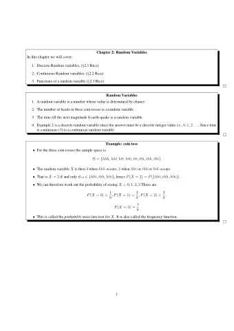


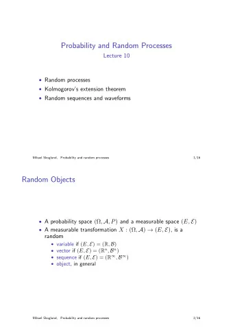
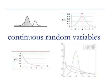


![arXiv:1708.08296v1 [cs.AI] 28 Aug 2017 ABSTRACT were crucial factors to success. Todays](https://c.sambuz.com/709961/arxiv-1708-08296v1-cs-ai-28-aug-2017-s.webp)


More recommend
Explore More Topics
Stay informed with curated content and fresh updates.