(R)NN-based Language Models Lecture 12 CS 753 Instructor: Preethi - PowerPoint PPT Presentation
(R)NN-based Language Models Lecture 12 CS 753 Instructor: Preethi Jyothi Word representations in Ngram models In standard Ngram models, words are represented in the discrete space involving the vocabulary Limits the possibility of truly
(R)NN-based Language Models Lecture 12 CS 753 Instructor: Preethi Jyothi
Word representations in Ngram models In standard Ngram models, words are represented in the • discrete space involving the vocabulary Limits the possibility of truly interpolating probabilities of • unseen Ngrams Can we build a representation for words in the continuous • space?
Word representations 1-hot representation: • Each word is given an index in {1, … , V}. The 1-hot vector • f i ∈ R V contains zeros everywhere except for the i th dimension being 1 1-hot form, however, doesn’t encode information about word • similarity Distributed (or continuous) representation: Each word is associated • with a dense vector. Based on the “distributional hypothesis”. E.g. dog → {-0.02, -0.37, 0.26, 0.25, -0.11, 0.34}
Word embeddings These distributed representations in a continuous space are • also referred to as “word embeddings” Low dimensional • Similar words will have similar vectors • Word embeddings capture semantic properties (such as • man is to woman as boy is to girl, etc.) and morphological properties (glad is similar to gladly, etc.)
Word embeddings [C01]: Collobert et al.,01
Relationships learned from embeddings [M13]: Mikolov et al.,13
Bilingual embeddings [S13]: Socher et al.,13
Word embeddings These distributed representations in a continuous space are • also referred to as “word embeddings” Low dimensional • Similar words will have similar vectors • Word embeddings capture semantic properties (such as • man is to woman as boy is to girl, etc.) and morphological properties (glad is similar to gladly, etc.) The word embeddings could be learned via the first layer of • a neural network [B03]. [B03]: Bengio et al., “A neural probabilistic LM”, JMLR, 03
Word embeddings Introduced the architecture that • forms the basis of all current neural language and word embedding models Embedding layer • One or more middle/hidden layers • Softmax output layer • [B03]: Bengio et al., “A neural probabilistic LM”, JMLR, 03
Continuous space language models Neural Network output input probability estimation layer is p 1 = w j n + 1 − projection fully-connected P ( w j = 1 | h j ) layer hidden layer to p i = M oi 1 P ( w j = i | h j ) , V cl dj w j shared n + 2 posterior − projections H w j P 1 − p N = (2) P ( w j = N | h j ) N N input discrete LM probabilities continuous ord representation: representation: for all words indices in wordlist P dimensional vectors ele- [S06]: Schwenk et al., “Continuous space language models for SMT”, ACL, 06
NN language model Neural Network output input probability estimation layer is p 1 = w j n + 1 Project all the words of the • − projection fully-connected P ( w j = 1 | h j ) layer hidden context h j = w j-n+1 ,…,w j-1 to layer to p i = their dense forms M oi 1 P ( w j = i | h j ) , V cl dj Then, calculate the • w j shared n + 2 posterior − projections language model probability H Pr(w j =i| h j ) for the given w j P 1 − p N = context h j (2) P ( w j = N | h j ) N N input discrete LM probabilities continuous ord representation: representation: for all words indices in wordlist P dimensional vectors ele-
NN language model Neural Network Dense vectors of all the words in • output input probability estimation layer context are concatenated forming is p 1 = w j the first hidden layer of the neural n + 1 − projection fully-connected P ( w j = 1 | h j ) layer hidden network layer to p i = M Second hidden layer: • oi 1 P ( w j = i | h j ) , V cl dj d j = tanh( Σ m jl c l + b j ) ∀ j = 1, …, H w j shared n + 2 posterior − projections Output layer: • H w j P 1 − p N = o i = Σ v ij d j + b’ i ∀ i = 1, …, N (2) P ( w j = N | h j ) N N p i → softmax output from the ith • input neuron → Pr(w j = i | h j ) discrete LM probabilities continuous ord representation: representation: for all words indices in wordlist P dimensional vectors ele-
NN language model Model is trained to minimise the following loss function: • X ! N X X m 2 v 2 L = t i log p i + ✏ kl + ik i =1 kl ik Here, t i is the target output 1-hot vector (1 for next word in • the training instance, 0 elsewhere) First part: Cross-entropy between the target distribution and • the distribution estimated by the NN Second part: Regularization term •
Decoding with NN LMs Two main techniques used to make the NN LM tractable for • large vocabulary ASR systems: 1. Lattice rescoring 2. Shortlists
Use NN language model via lattice rescoring Lattice — Graph of possible word sequences from the ASR system using an • Ngram backoff LM Each lattice arc has both acoustic/language model scores. • LM scores on the arcs are replaced by scores from the NN LM •
Decoding with NN LMs Two main techniques used to make the NN LM tractable for • large vocabulary ASR systems: 1. Lattice rescoring 2. Shortlists
Shortlist Softmax normalization of the output layer is an expensive • operation esp. for large vocabularies Solution: Limit the output to the s most frequent words. • LM probabilities of words in the short-list are calculated by • the NN LM probabilities of the remaining words are from Ngram • backoff models
Results Table 3 Perplexities on the 2003 evaluation data for the back-o ff and the hybrid LM as a function of the size of the CTS training data CTS corpus (words) 7.2 M 12.3 M 27.3 M In-domain data only Back-o ff LM 62.4 55.9 50.1 Hybrid LM 57.0 50.6 45.5 Interpolated with all data Back-o ff LM 53.0 51.1 47.5 Hybrid LM 50.8 48.0 44.2 28 backoff LM, CTS data hybrid LM, CTS data System 1 Eval03 word error rate backoff LM, CTS+BN data 26 hybrid LM, CTS+BN data 25.27% 24.51% 24.09% 24 System 2 23.70% 23.04% 22.32% 22.19% 22 21.77% System 3 20 19.94% 19.30% 19.10% 18.85% 18 7.2M 12.3M 27.3M in-domain LM training corpus size [S07]: Schwenk et al., “Continuous space language models”, CSL, 07
word2vec (to learn word embeddings) Continuous bag-of-words Skip-gram CBOW Image from: Mikolov et al., “Efficient Estimation of Word Representations in Vector Space”, ICLR 13
Bias in word embeddings Image from:http://wordbias.umiacs.umd.edu/
Longer word context? What have we seen so far: A feedforward NN used to • compute an Ngram probability Pr(w j = i ∣ h j ) (where h j encodes the Ngram history) We know Ngrams are limiting: • Alice who had attempted the assignment asked the lecturer How can we predict the next word based on the entire • sequence of preceding words? Use recurrent neural networks (RNNs)
Simple RNN language model OUTPUT(t) INPUT(t) Current word, x t • CONTEXT(t) Hidden state, s t Output, y t U V s t = f ( Ux t + Ws t − 1 ) o t = softmax( V s t ) RNN is trained using the • W cross-entropy criterion CONTEXT(t-1) Image from: Mikolov et al., “Recurrent neural network based language model”, Interspeech 10
RNN-LMs Optimizations used for NNLMs are relevant to RNN-LMs as • well (rescoring Nbest lists or lattices, using a shortlist, etc.) Perplexity reductions over Kneser-Ney models: • Model # words PPL WER KN5 LM 200K 336 16.4 KN5 LM + RNN 90/2 200K 271 15.4 KN5 LM 1M 287 15.1 KN5 LM + RNN 90/2 1M 225 14.0 KN5 LM 6.4M 221 13.5 KN5 LM + RNN 250/5 6.4M 156 11.7 Image from: Mikolov et al., “Recurrent neural network based language model”, Interspeech 10
LSTM-LMs Vanilla RNN-LMs • unlikely to show full potential of recurrent models due to issues like vanishing gradients LSTM-LMs: Similar • to RNN-LMs except use LSTM units in the 2nd hidden (recurrent) layer Image from: Sundermeyer et al., “LSTM NNs for Language Modeling”, IS 10
Comparing RNN-LMs with LSTM-LMs Sigmoid 160 LSTM 150 PPL 140 130 120 50 100 150 200 250 300 350 Hidden layer size Image from: Sundermeyer et al., “LSTM NNs for Language Modeling”, 10
Character-based RNN-LMs Image from: http://karpathy.github.io/2015/05/21/rnn-effectiveness/ Good tutorial available at https://github.com/yunjey/pytorch-tutorial/blob/master/tutorials/02-intermediate/language_model/main.py#L30-L50
Generate text using a trained character-based LSTM-LM VIOLA: Why, Salisbury must find his flesh and thought That which I am not aps, not a man and in fire, To show the reining of the raven and the wars To grace my hand reproach within, and not a fair are hand, That Caesar and my goodly father's world; When I was heaven of presence and our fleets, We spare with hours, but cut thy council I am great, Murdered and by thy master's ready there My power to give thee but so much as hell: Some service in the noble bondman here, Would show him to her wine. Image from: http://karpathy.github.io/2015/05/21/rnn-effectiveness/
Recommend
More recommend
Explore More Topics
Stay informed with curated content and fresh updates.





![A PROPOSAL FOR THE CFT DUAL OF ADS3 AT THE STRING SCALE BASED ON arxiv:1803.04420 [hep-th] AND](https://c.sambuz.com/936966/a-proposal-for-the-cft-dual-of-ads3-at-the-string-scale-s.webp)
