Query Processing Query Processing Steps balance < 2500 ( - PowerPoint PPT Presentation
Query Processing Query Processing Steps balance < 2500 ( balance ( account)) balance ( balance < 2500 ( account)) Step 1 SELECT balance FROM account WHERE balance < 2500 Step 2 Step 3 A B + -tree index on balance
Query Processing
Query Processing Steps σ balance < 2500 ( ∏ balance ( account)) ∏ balance ( σ balance < 2500 ( account)) Step 1 SELECT balance FROM account WHERE balance < 2500 Step 2 Step 3 A B + -tree index on balance CMPT 454: Database II -- Query Processing 2
Query Cost Measures • Query processing as an optimization problem – Search space: all possible equivalent relational algebra expressions � all possible query execution plans – Goal: find the most efficient query execution • Efficiency: I/O or CPU? – CPU processing time is often much smaller than I/O cost, and is hard to estimate (real systems do consider) – Each I/O access cost may slightly different – Number of block transfers is a measure of the dominant component of query answering cost – Communication cost in distributed database systems CMPT 454: Database II -- Query Processing 3
Selection • Table-scan: read the blocks one by one from disk – Linear search: scan each file block, • Cost = t S + b r * t T , where b r is the number of blocks in the file, t S is the average seek time, and t T is the average block transfer time • Search on a key attribute: an average cost of b r / 2 • Can be used in any cases – Binary search: the file is ordered on an attribute, the selection condition is an equality comparison on the attribute • Cost: ⎡ log 2 (b r ) ⎤ * (t S + t T ) • If the attribute is not a key, some extra blocks may need to be read • Index-scan: using an index in selection – Primary index, equality on key: if a B+-tree is used, (h i + 1) * (t S + t T ), where h i is the height of the tree – Primary index, equality on nonkey: h i * ( t T + t S ) + t S + t T * b, where b is the number of blocks containing records with the specified search key – Secondary index, equality on key: (h i + 1) * (t S + t T ) – Secondary index, equality on nonkey: ( h i + n) * ( t T + t S ), can be worse than linear search CMPT 454: Database II -- Query Processing 4
Selection Involving Comparisons • Primary index, comparison – Case A > v or A ≥ v: use the index to find the first tuple having A ≥ v, scan the tuple up to the end of the file, cost h i * ( t T + t S ) + t S + t T * b – Case A < v or A ≤ v: scan from the beginning of the file until the condition is violated, the index is not used • Secondary index, comparison: use the index to find the pointers to the record, retrieve the data blocks – Sort pointers to ensure each block is read once – Can be costly if the selectivity of a query is low (i.e., many tuples satisfy the condition) • Conjunction σ θ 1 ∧ θ 2 ∧ . . . θ n ( r) – Selection and test using one index on one attribute of composite search key – Selection by intersection of identifiers • Disjunction σ θ 1 ∨ θ 2 ∨ . . . θ n ( r) by union of identifiers CMPT 454: Database II -- Query Processing 5
Nested-Loop Join • To compute the theta join r θ s for each tuple t r in r do begin for each tuple t s in s do begin test whether pair ( t r ,t s ) satisfies the join condition θ if so, add t r • t s to the result end end – r : the outer relation of the join – s : the inner relation of the join • No indexes, can be used with any kind of join condition • Cost – Worst case – only one block of each relation in memory: n r ∗ b s + b r – Best case: both relations are in memory: b r + b s – If one relation can fit entirely in main memory, use that relation as the inner relation: b r + b s CMPT 454: Database II -- Query Processing 6
Block Nested-Loop Join • Idea: once a block is read into main memory, the records in the block should be utilized as much as possible for each block B r of r do begin for each block B s of s do begin for each tuple t r in B r do begin for each tuple t s in B s do begin check if ( t r ,t s ) satisfies the join condition if so, add t r • t s to the result end end end end • Cost – Worst case – only one block for each relation : b r ∗ b s + b r – Best case: b r + b s CMPT 454: Database II -- Query Processing 7
Further Improvements • In natural join or equi-join, if the join attributes form a key on the inner relation, then for each outer relation tuple, the inner loop can stop as soon as the first match is found • In the block nested-loop algorithm, if M blocks are available, use M-2 blocks for outer relation (why?) – Total cost: ⎡ b r / (M-2) ⎤ ∗ b s + b r • Scan the inner loop alternately forward and backward (similar to the elevator algorithm), reuse the blocks remaining in the buffer – How and why is it good? • Indexed nested-loop join – An index exists on the inner loop’s join attribute – use the index lookups to replace file scans – Cost: b r ( t T + t S ) + n r ∗ c, w here c is the cost of a single selection on s using the join condition, n r is the number of records in r • If indices are available on the join attributes of both r and s, use the relation with fewer tuples as the outer relation CMPT 454: Database II -- Query Processing 8
Merge Join • Can be used only for equi-joins and natural joins • Sort both relations on their join attribute (if not already sorted on the join attributes) • Merge the sorted relations to join them – Join step is similar to the merge stage of the sort-merge algorithm – Every pair with same value on join attribute must be matched Cost: b r + b s block transfers + ⎡ b r / b b ⎤ + ⎡ b s / b b ⎤ • seeks + the cost of sorting if relations are unsorted – After sorting, each block needs to be read only once – Suppose all tuples for any given value of the join attributes fit in memory – Can be further improved by combining the merge phase of merge-sort with the merge phase of merge- join – merge-join multiple sorted sublists CMPT 454: Database II -- Query Processing 9
Hash Join: the Idea CMPT 454: Database II -- Query Processing 10
Hash Join • For equi-joins and natural joins only • A hash function h depending only on the join attributes is used to partition tuples of both relations, – h maps JoinAttrs values to {0, 1, ..., n } – r 0 , r 1 , . . ., r n are partitions of r tuples, each tuple t r ∈ r is put in partition r i where i = h(t r [JoinAttrs]) – s 0 ,, s 1 . . ., s n are partitions of s tuples, each tuple t s ∈ s is put in partition s i , where i = h(t s [JoinAttrs]) – r tuples in r i need only to be compared with s tuples in s i CMPT 454: Database II -- Query Processing 11
Setting Parameters of Hash Joins • Algorithm: relation s : build input, relation r : probe input Partition the relation s using hashing function h, w hen partitioning a relation, one block of memory is reserved as the output buffer for each partition Partition r similarly For each i do Load s i into memory and build an in-memory hash index on it using the join attribute This hash index uses a different hash function than the earlier one h Read the tuples in r i from the disk one by one For each tuple t r locate each matching tuple t s in s i using the in-memory hash index Output the concatenation of their attributes • n and the hash function h is chosen such that each s i should fit in memory – Use the smaller input relation as the build relation – The probe relation partitions r i need not fit in memory Typically n is chosen as ⎡ b s /M ⎤ * f where f is a “fudge factor”, typically around • 1.2 CMPT 454: Database II -- Query Processing 12
Recursive Partitioning, Overflow • For number of partitions n is greater than number of pages M of memory, instead of partitioning n ways, use M – 1 partitions for s • Further partition the M – 1 partitions using a different hash function, use same partitioning method on r (Rarely required) • Hash table overflow: a partition cannot fit in memory – Many tuples with same value for join attributes due to bad hash function – Partitioning is said skewed if some partitions have significantly more tuples than some others • Overflow resolution in build phase – Partition s i is further partitioned using different hash function – Partition r i must be similarly partitioned • Overflow avoidance – Performs partitioning carefully to avoid overflows during build phase – E.g. partition build relation into many partitions, then combine them • Both approaches fail with large numbers of duplicates – Fallback option: use block nested loops join on overflowed partitions CMPT 454: Database II -- Query Processing 13
Performance Analysis • Without recursive partitioning: 3 ( b r + b s ) + 4 ∗ n h • For recursive partitioning: 2 (b r + b s ) ⎡ log M– 1 ( b s ) – 1 ⎤ + b r + b s – Cost of partitioning s : ⎡ log M– 1 ( b s ) – 1 ⎤ – Similar cost for partitioning r – best to choose the smaller relation as the build relation • If the entire build input can be kept in main memory, then do not partition the relations into temporary files – Cost: b r + b s CMPT 454: Database II -- Query Processing 14
Hybrid Hash Join • Join the first partitions during partitioning the tables – Partition relation s, keep the first partition s 0 in main memory – Partition relation r, join tuples in r 0 with s 0 in main memory – No need to store s 0 and r 0 • Most useful if M >> b s CMPT 454: Database II -- Query Processing 15
Recommend
More recommend
Explore More Topics
Stay informed with curated content and fresh updates.

