Quelques applications de l’in´ egalit´ e de Lojasiewicz ` a des discr´ etisations d’EDP Morgan PIERRE Laboratoire de Math´ ematiques et Applications, UMR CNRS 6086, Universit´ e de Poitiers , France SMAI 2011, 23-27 mai 2011 Morgan PIERRE SMAI 2011
Consider the gradient flow U ′ ( t ) = −∇ F ( U ( t )) t ≥ 0 , (1) where U = ( u 1 , . . . , u d ) t , F ∈ C 1 , 1 loc ( R d , R ). For every solution U ( t ), we have � t � U ′ ( s ) � 2 ds = F ( U (0)) , F ( U ( t )) + t ≥ 0 . 0 If U is a solution of (1) which is bounded on [0 , + ∞ ), then ω ( U (0)) := { U ⋆ : ∃ t n → + ∞ , U ( t n ) → U ⋆ } is a non-empty compact connected subset of S = { V ∈ R d : ∇ F ( V ) = 0 } . � � Moreover, d U ( t ) , ω ( U (0)) → 0 as t → + ∞ . Morgan PIERRE SMAI 2011
Does U ( t ) → U ⋆ as t → + ∞ ? If d = 1, it is obvious by monotonicity. If d ≥ 2, it is obviously true if S is discrete, but it is no longer true in general: counterexample in Palis and De Melo’82. The following counter-example is given in Absil, Mahony and Andrews’05 : 4 r 4 � 1 � F ( r , θ ) = e − 1 / (1 − r 2 ) 1 − 4 r 4 + (1 − r 2 ) 4 sin( θ − 1 − r 2 ) , if r < 1 and F ( r , θ ) = 0 otherwise. We have F ∈ C ∞ , F ( r , θ ) > 0 for r < 1 so every point on the circle r = 1 is a global minimizer. We can check that the curve defined by θ = 1 / (1 − r 2 ) is a trajectory. Morgan PIERRE SMAI 2011
0.4 1.5 1 0.3 0.5 0.2 0 0.1 −0.5 −1 0 x 1.5 −1.5 1 0.5 0 −0.5 −1 −1.5 y “Mexican hat” function Morgan PIERRE SMAI 2011
Theorem (Lojasiewicz’65) If F : R d → R is real analytic in a neighbourhood of U ∈ R d , there exist ν ∈ (0 , 1 / 2] , σ > 0 and γ > 0 s.t. for all V ∈ R d , � V − U � < σ ⇒ | F ( V ) − F ( U ) | 1 − ν ≤ γ �∇ F ( V ) � . (2) Morgan PIERRE SMAI 2011
Theorem (Lojasiewicz’65) If F : R d → R is real analytic in a neighbourhood of U ∈ R d , there exist ν ∈ (0 , 1 / 2] , σ > 0 and γ > 0 s.t. for all V ∈ R d , � V − U � < σ ⇒ | F ( V ) − F ( U ) | 1 − ν ≤ γ �∇ F ( V ) � . (2) Example: for d = 1 and p ≥ 2, x �→ | x | p satisfies (2) at x = 0 with ν = 1 / p . Also true for 1 < p ≤ 2. In the ”generic case”’ where ∇ 2 F ( U ) inversible, ν = 1 / 2. for d = 1, the C ∞ function Counter-examples: x �→ exp( − 1 / x 2 ) satisfies (2) at x = 0 for ν = 0 (too weak). The C ∞ function x �→ exp( − 1 / x 2 ) sin(1 / x ) does not satisfy (2) at x = 0. NB: see the preprint of Michel Coste on his web page. Morgan PIERRE SMAI 2011
Corollary If F : R d → R is real analytic, then for any bounded semi-orbit of U ′ ( t ) = −∇ F ( U ( t )) , there exists U ∞ ∈ S s.t. U ( t ) → U ∞ as t → + ∞ . Moreover , let ν be a Lojasiewicz exponent of F at U ∞ : • if ν = 1 / 2 , then for t large enough, F ( U ( t )) ≤ Ce − α t and � U ( t ) − U ∞ � ≤ C ′ e − α t / 2 , for some constants α , C and C ′ > 0 ; • if ν ∈ (0 , 1 / 2) , then for t large enough F ( U ( t )) ≤ Ct − 1 / (1 − 2 ν ) and � U ( t ) − U ∞ � ≤ C ′ t − ν/ (1 − 2 ν ) , for some constants C and C ′ > 0 . NB : optimal convergence rates. If F ( x ) = | x | p ( p > 2), then ν = 1 / p , ν/ (1 − 2 ν ) = 1 / ( p − 2) and the solution of x ′ ( t ) = −| x ( t ) | p − 1 is C p ( C + t ) 1 / (2 − p ) . Morgan PIERRE SMAI 2011
A proof (convergence) − [ F ( U ( t )) ν ] ′ − ν U ′ ( t ) · ∇ F ( U ( t )) F ( U ( t )) ν − 1 = ν � U ′ ( t ) ��∇ F ( U ( t )) � F ( U ( t )) ν − 1 = νγ − 1 � U ′ ( t ) � , ≥ � t F ( U ( t n )) ν − F ( U ( t )) ν ≥ νγ − 1 � U ′ ( s ) � ds . so t n Morgan PIERRE SMAI 2011
A proof (convergence) F ( U ( t )) is non increasing and so has a limit F ⋆ (= 0). Let t n → + ∞ s.t. U ( t n ) → U ⋆ . We have F ( U ⋆ ) = F ⋆ and U ⋆ ∈ S . Choose n large enough so that � U ( t n ) − U ⋆ � < σ/ 2 and ν − 1 γ F ( U ( t n )) ν < σ/ 2, and define t + = sup { t ≥ t n | � U ( s ) − U ⋆ � < σ ∀ s ∈ [ t n , t ) } . For t ∈ [ t n , t + ), we have − [ F ( U ( t )) ν ] ′ − ν U ′ ( t ) · ∇ F ( U ( t )) F ( U ( t )) ν − 1 = ν � U ′ ( t ) ��∇ F ( U ( t )) � F ( U ( t )) ν − 1 = νγ − 1 � U ′ ( t ) � , ≥ � t F ( U ( t n )) ν − F ( U ( t )) ν ≥ νγ − 1 � U ′ ( s ) � ds . so t n Thus � U ( t ) − U ( t n ) � < σ/ 2, ∀ t ∈ [ t n , t + ) and so t + = + ∞ , otherwise � U ( t + ) − U ⋆ � = σ and � U ( t + ) − U ⋆ � ≤ � U ( t + ) − U ( t n ) � + � U ( t n ) − U ⋆ � < σ, a contradiction. QED. Morgan PIERRE SMAI 2011
Questions: If we consider (stable) time discretizations of the gradient flow, can we obtain similar results of convergence to equilibrium ? In particular, what happens for the backward Euler scheme ? What restriction on the time step do we have ? Can we find a unifying background ? Morgan PIERRE SMAI 2011
The backward Euler scheme for (1) reads: let U 0 ∈ R d , and for n ≥ 0, let U n +1 solve U n +1 − U n = −∇ F ( U n +1 ) , (3) ∆ t where ∆ t > 0 is fixed and F ∈ C 1 ( R d , R ). Since existence is not obvious, we rewrite (3) in the form: � � V − U n � 2 � U n +1 ∈ argmin + F ( V ) : V ∈ R d . (4) 2∆ t In optimization, (4) is known as the proximal algorithm . In particular, U n +1 satisfies 1 2∆ t � U n +1 − U n � 2 ≤ F ( U n ) . F ( U n +1 ) + Morgan PIERRE SMAI 2011
By induction, any sequence defined by (4) satisfies n − 1 1 � U k +1 − U k � 2 ≤ F ( U 0 ) , � F ( U n ) + ∀ n ≥ 0 (5) 2∆ t k =0 This is a stability result. By (5), it is easy to prove that if ( U n ) n ∈ N is a bounded sequence defined by the proximal algorithm (4), then � U ⋆ ∈ R d : ∃ n k → + ∞ , U n k → U ⋆ � ω ( U 0 ) := is a non-empty compact connected subset of S . Moreover, d ( U n , ω ( U 0 )) → 0 as n → + ∞ . Question : does U n → U ⋆ as n → + ∞ ? Morgan PIERRE SMAI 2011
Theorem (Attouch and Bolte’09, Merlet and P.’10) If F : R d → R is real analytic, and if ( U n ) n is a bounded sequence defined by the proximal algorithm (4) , then there exists U ∞ ∈ S s.t. U n → U ∞ as n → + ∞ . Morgan PIERRE SMAI 2011
Theorem (Attouch and Bolte’09, Merlet and P.’10) If F : R d → R is real analytic, and if ( U n ) n is a bounded sequence defined by the proximal algorithm (4) , then there exists U ∞ ∈ S s.t. U n → U ∞ as n → + ∞ . Remark 1: If lim � V �→ + ∞ F ( V ) = + ∞ , then ( U n ) n defined by (4) is bounded. Remark 2: A more general version: variable stepsize 0 < ∆ t ⋆ ≤ ∆ t n ≤ ∆ t ⋆ < + ∞ F : R d → R real analytic replaced by F : dom ( F ) ⊂ R d → R continuous and satisfies a Lojasiewicz property Remark 3: in addition, (optimal) convergence rates Morgan PIERRE SMAI 2011
The proof of convergence extends to many situations: For any other scalar product on R d : AU ′ ( t ) = −∇ F ( U ( t )) , where A is positive definite (symmetric or not). Generalizations in infinite dimension (Simon, Jendoubi, Haraux, Chill,. . . ) Semilinear heat equation: u t = ∆ u − f ( u ) , t ≥ 0 , x ∈ Ω Cahn-Hilliard equation (Hoffman, Rybka, Chill, Jendoubi): u t = − α ∆ 2 u + ∆ f ′ ( u ) , t ≥ 0 , x ∈ Ω , with f ′ ( u ) = u 3 − u typically, α > 0, and Neumann or periodic BC. Merlet and P.’10 Cahn-Hilliard equation with dynamic boundary conditions (Wu, Zheng, Chill, Fasangova, Pruss) Cherfils, Petcu and P.’10 Cahn-Hilliard-Gurtin equations (Miranville and Rougirel): gradient-like flow Injrou and P.’10 Morgan PIERRE SMAI 2011
Generalization to second-order gradient-like asymptotically autonomous flows: ǫ U ′′ ( t ) + U ′ ( t ) = −∇ F ( U ( t )) + G ( t ) , t ≥ 0 , where ǫ > 0 and G ( t ) − ∞ 0 fast enough: Haraux and → Jendoubi’98, Chill and Jendoubi’03, Grasselli and P., to appear Asymptotically autonomous damped wave equation ǫ u tt + u t = ∆ u − f ( u ) + g ( t ) , t ≥ 0 , x ∈ Ω . Haraux, Jendoubi, Chill,. . . Cahn-Hilliard equation with inertial term (Grasselli, Schimperna, Zelig, Miranville, Bonfoh) Grasselli, Lecoq and P., to appear (optimal) convergence rates for 1st and 2nd order Morgan PIERRE SMAI 2011
Application : Allen-Cahn equation u t ( x , t ) = α ∆ u ( x , t ) − f ′ ( u ( x , t )) , t ≥ 0 , x ∈ Ω , where Ω is bounded with Lipschitz boundary, α > 0, f ′ ( u ) = u 3 − u and Neumann boundary condition. It is a L 2 (Ω) gradient flow of the functional α � 2 |∇ u ( x ) | 2 + f ( u ( x )) dx . E ( u ) = Ω NB: +1, − 1 and 0 are steady states ; if Ω = unit disc and α > 0 small, there is a continuum of steady states . Morgan PIERRE SMAI 2011
A space discretization by finite elements with a nodal basis ( ϕ i ) i reads MU ′ ( t ) = − AU ( t ) − ∇ F h ( U ) , (6) where M = ( ϕ i , ϕ j ) i , j is the mass matrix, A = ( ∇ ϕ i , ∇ ϕ j ) i , j is the discrete Laplacian, and � � ∇ F h ( U ) i = f ′ ( u i ϕ i ( x )) ϕ i ( x ) dx , Ω i is the gradient of F h ( U ) = � Ω f ( � i u i ϕ i ( x )) dx . (6) is a gradient flow , so we have convergence to equilibrium for its time discretization (by the backward Euler scheme). A similar argument holds for the standard finite difference scheme. Morgan PIERRE SMAI 2011
Recommend
More recommend
Unleash a World of Digital Possibilities—Browse, Share, and Explore Content Without Boundaries