Quantum Benchmarks for Gaussian States J. Calsamiglia M. Aspachs - PowerPoint PPT Presentation

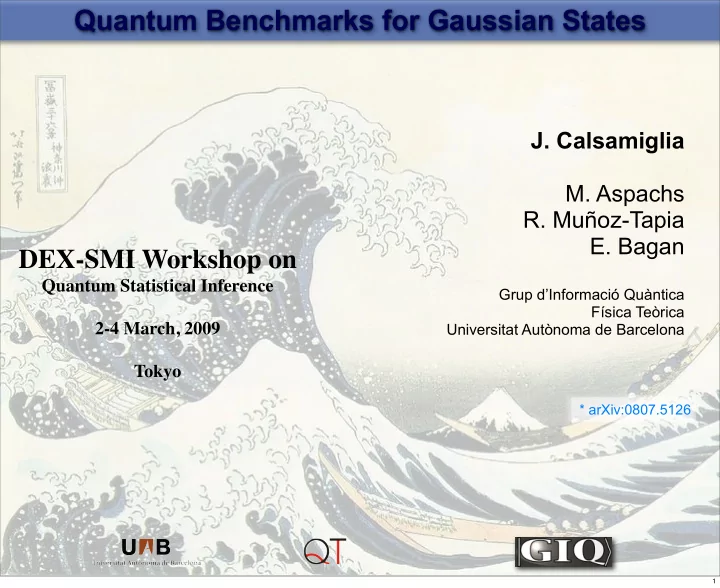
Quantum Benchmarks for Gaussian States J. Calsamiglia M. Aspachs R. Muñoz-Tapia E. Bagan DEX-SMI Workshop on Quantum Statistical Inference Grup d’Informació Quàntica Física Teòrica 2-4 March, 2009 Universitat Autònoma de Barcelona Tokyo * arXiv:0807.5126 1

Gaussian States • A family of continuos variable quantum states defined by a Gaussian characteristic function. • Canonical form: ρ = D ( α ) S ( r, φ ) ρ β S ( r, φ ) † D ( α ) † e − β ˆ n D ( α ) = e α a † − α ∗ a r/ 2( a 2 e − i 2 φ − a † 2 e i 2 φ ) � � ρ β = S ( r, φ ) = exp tr (e − β ˆ n ) • Very good description of states of light produced in labs (laser produces coherent state + passive/active optical operations) 2

Quantum Benchmarks IDEAL identity channel ρ ( ρ ( e.g. quantum teleportation = E ( ρ ) or quantum memories REAL noisy identity channel ? ρ ( ˜ e.g. quantum teleportation E ( ρ ) or quantum memories Are quantum resources necessary to emulate the channel? 3

Are quantum resources necessary to emulate the channel? First threshold for quantum teleportation of coherent states: Fidelity of output state when no quantum correlations are used. F tel = � α | ρ out | α � = �� � d β 2 tr( E β | α � = � α | � α | ) | β � � β | | α � = � � d 2 β e − 2 | α − β | 2 = 1 = 1 d 2 β | � α | β � | 4 = 1 π π 2 where E β = 1 π | β � � β | Quantum resources F = � α | ρ out | α � > 1 / 2. are being used. A. Furusawa et. al. Science 1998 4

More rigorous quantum benchmark (Braunstein, Fuchs & Kimble JMO 2000) : VM, { O χ } , † ( ) = � ρ out = tr( ρ in O χ ) ρ χ χ ρ in ∈ Ω χ Measure + Prepare � F = � ψ in | ρ out | ψ in � P ( | ψ in � ) d | ψ in � Different choices of input-state families: x = � ψ 0 | ψ 1 � F = 1 � � � 1 − x 2 + x 4 • 2 non-orthogonal states: , 1 + ≥ 0 . 933 and | ψ 1 � , | ψ 0 � 2 2 d →∞ • Isotropic distribution (all pure states with equal probability): F = − → 0 d + 1 • Coherent states with Gaussian distribution of amplitudes: (Braunstein, et al.) are coherent states F coh = 1 + λ π e − λ | α | 2 . λ → 0 p ( α ) = λ − → 1 / 2 2 + λ Hammerer et. al. PRL 2005 • Micro-canonical ensemble of pure Gaussian states (Serafini et al PRL 2007) 5

We consider Gaussian phase-covariant family of input states: ρ φ in = U ( φ ) ρ 0 U ( φ ) † φ ∈ [0 , 2 π ) where is a Gaussian state (pure or mixed) ρ 0 U ( φ ) = e i φ a † a and � d φ 2 π F ( ρ φ in , ρ φ • Benchmark F cl = av ) F ( ρ 1 , ρ 2 ) = (tr | √ ρ 1 √ ρ 2 | ) 2   χ p ( χ | ρ φ ρ φ av = � in ) ρ χ  6

• Phase-covariant family is large enough to give reasonable benchmarks, and is easy to produce experimentally. Adesso & Chiribella [PRL 2008] have also studied benchmarks with • ρ ( r ) = ˆ S ( r ) ρ β ˆ S ( r ) † mixed states taking as input family: � � F AC = drP ( r ) p ( χ | r ) F [ ρ ( r ) , ρ ( r χ )] ≤ χ � � drP ( r ) F [ ρ ( r ) , p ( χ | r ) ρ ( r χ )] = F cl ≤ fidelity is concave χ - Optimal Guess typically does not belong to family of input states. - Difficult to change squeezing parameter experimentally. ✴ Recently: phase covariant and displaced squeezed states (Owari et al.) 7

• Covariant strategies Given a strategy one can define a phase-shifted strategy by { O χ = | ξ χ � � ξ χ | , ρ χ } O χ , θ = U θ O χ U † θ , ρ χ , θ = U θ ρ χ U † with at least the same fidelity: θ 1 � F θ = d φ F ( ρ φ , ρ φ , θ av ) = 2 π 2 � �   � � �� � √ ρ 0 U † tr( U θ [ ξ χ ] U † θ U φ ρ 0 U † φ ) ρ χ U † � � =  tr = d φ U φ φ U θ � �  θ � � χ � � � av ) = F ( θ =0) d ϕ F ( ρ ϕ , ρ ϕ = tr | UBV | = tr | B | ϕ = φ − θ where we have used the notation [ ψ ] = | ψ � � ψ | 8

• Covariant strategies Given set one can define a covariant strategy by { O χ = | ξ χ � � ξ χ | , ρ χ } O χ , θ = 1 / (2 π ) U θ O χ U † θ , ρ χ , θ = U θ ρ χ U † with at least the same fidelity: θ fidelity is concave � � � � � F cl = F θ = 1 / 2 π d θ F θ ≤ ρ φ , 1 / 2 π d θρ φ , θ ≡ F cov d φ F av � where ρ φ , θ p ( χ θ | ρ φ ) ρ χ , θ av = χ �� d θ � 2 � � � � � � F cov = √ ρ 0 U † � tr( U θ [ ξ χ ] U † θ U φ ρ 0 U † φ ) U θ ρ χ U † tr = d φ � U φ � � φ θ 2 π � � � χ �� d ϕ � 2 � � � � 2 � � � � � � tr( U ϕ [ ξ χ ] U † ϕ ρ 0 ) U ϕ ρ χ U † � = tr = tr ρ 0 √ ρ av √ ρ 0 � � � � ϕ 2 π � � � � � � χ � � where ρ av = p ( χ θ | ρ 0 ) ρ χ , θ d θ χ 9

The optimal classical fidelity (or quantum benchmark) can be conveniently written as, � √ ρ av | ) 2 � with F =(tr | √ ρ 0 ρ av = p ( χ , θ | ρ 0 ) ρ χ , θ d θ χ Note that for a single seed, the completeness relation fixes the POVM: O θ = 1 2 π U θ [ ξ ] U † � (up to some arbitrary phases) θ with | ξ � = | n � n The fidelity can be conveniently written as, � 2 � √ ρ 0 ⊗ √ ρ 0 K √ ρ 0 ⊗ √ ρ 0 � F = max tr B tr A K � � with ρ av = tr A ( ρ 0 ⊗ 1 1 K ) K = d θ O χ , θ ⊗ ρ χ , θ χ θ tr B K = I A ( U θ ⊗ U θ tr i.e., , , invariant & separable. maximization over the maximization 10

• For pure states: ρ 0 = | ψ 0 � � ψ 0 | F = � ψ 0 | � ψ 0 | K | ψ 0 � | ψ 0 � Navascues PRL 2008 Also, for fixed POVM with seeds the optimal fidelity can be written as, {| ξ χ � � ξ χ |} � � � with d φ / (2 π ) | � ξ χ | ψ φ � | 2 | ψ φ �� ψ φ | F = � ψ χ | A χ | ψ χ � = � A χ � ∞ A χ = sup ψ χ χ χ � d φ with 2 π | ψ φ � | ψ φ �� ψ φ | � ψ φ | Λ = A χ = � ξ χ | Λ | ξ χ � Hammerer PRL 2005 Optimal fidelity given by largest eigenvalue, and optimal guess given by corresponding eigenvector. • If one restricts the guess-states to be in the input ensemble , things also Ω simplify considerably. e.g. in the pure state case, the optimal POVM is known to be the single-seed POVM or canonical phase-measurement . | ξ � = � n | n � A. S. Holevo, Probab. & Stat. Aspects of Q. T., (1982) • In general, no assumptions about the POVM nor the guess can be made, and we have to resort on numerical methods. 11

Qubits Can be solved with full generality. � 2 � √ ρ 0 ⊗ √ ρ 0 K √ ρ 0 ⊗ √ ρ 0 � F = max tr B tr A K Input θ � 1+ r � 0 U † 2 ρ 0 = U y, θ 1 − r y, θ 0 2   a 0 0 0  K ≥ 0 ⇔ (1 − a )(1 − c ) ≥ | b | 2 , 0 ≤ a ≤ 1 , 0 ≤ c ≤ 1 0 1 − a b 0    K =   b 1 − c 0 0   K Γ ≥ 0 ⇔ ac − | b | 2 ≥ 0  c 0 0 0 Change inequalities to equalities at the expense of additional variables, (1 − a )(1 − c ) − | b | 2 = w 2 , ac − | b | 2 = u 2 Using Lagrange multipliers and after some algebraic manipulations we arrive to: a = cos 2 ζ  � r 2 sin 2 θ + (1 − r 2 )(4 − r 2 sin 2 θ )  c = sin 2 ζ ζ = arctan 2 r cos θ b = √ ac = 1 / 2 sin 2 ζ  12

• Optimal strategy given by single-seed covariant POVM   POVM-element guessed-state cos 2 ζ 2 sin ζ cos 2 ζ 1 1 2 sin ζ 2 2 � �� � 2 sin ζ sin 2 ζ 2 sin ζ sin 2 ζ 1 1 � �� �   � 0 | U † 2 | + � � + | ⊗ U y, ζ | 0 � 2 2 y, ζ =   cos 2 ζ 2 sin ζ cos 2 ζ 1 1 2 sin ζ   2 2 Guess 2 sin ζ sin 2 ζ 2 sin ζ sin 2 ζ 1 1 2 2 ζ Input cos 2 ζ   0 0 0 2 POVM sin 2 ζ 1 2 sin ζ 0 0   2 K =   2 sin ζ cos 2 ζ 1 0 0   2 sin 2 ζ * ) ( 0 0 0 d e e s - e l g 2 n i s t a h t e t a c i d n i s t u l s e r r a l o c f i n r e e m v u e , N 3 ≥ d r o f a l m i p t o t o n s i M V O P n t a i r a v o c ) . t g i i d d 3 r n i e c n e e r f f d i ( e a t s t e r u p � � � 1 + r cos θ F = 1 r 2 sin 2 θ + (1 − r 2 )(4 − r 2 sin 2 θ ) f o r e b m u n a l m i n m i e h t n o s d ζ = arctan n u o b n cos ζ w 2 o n k o N 2 r cos θ ) s d e e s o r ( s n t e m e l e M V O P • Single-seed POVM (canonical phase-measurement) is optimal (*!) • Guess does not belong to input family: - Guess is always pure. - Guess points in a different direction than input state. ζ ≤ θ 13

Qubits � � 1 + r cos θ F = 1 cos ζ 2 Guess Input � r 2 sin 2 θ + (1 − r 2 )(4 − r 2 sin 2 θ ) POVM ζ = arctan 2 r cos θ F = 1 • Pure states 8 [7 + cos(2 θ )] F = 1 � � 2 + r 2 + � • Equatorial plane 4 − 5 r 2 + r 4 4 F F Cl √ 2 π ( | 0 � + e i θ | 1 � } {| θ � = 1 / 1.00 • Continuos POVM overcomes 2-outcome S-G measurement. 0.95 0.90 √ where |± � = 1 / 2( | 0 � ±| 1 � ). • Mixedness improves classical Fidelity 0.85 Now we make use of (4.13) 0.80 r 0.2 0.4 0.6 0.8 1.0 14