Quantum algorithms for the subset-sum problem D. J. Bernstein - - PDF document

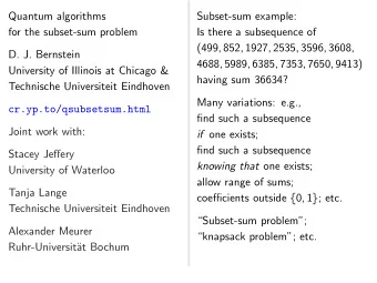
Quantum algorithms for the subset-sum problem

• D. J. Bernstein

University of Illinois at Chicago & Technische Universiteit Eindhoven cr.yp.to/qsubsetsum.html Joint work with: Stacey Jeffery University of Waterloo Tanja Lange Technische Universiteit Eindhoven Alexander Meurer Ruhr-Universit¨ at Bochum

Subset-sum example: Is there a subsequence of (499❀ 852❀ 1927❀ 2535❀ 3596❀ 3608❀ 4688❀ 5989❀ 6385❀ 7353❀ 7650❀ 9413) having sum 36634? Many variations: e.g., find such a subsequence if one exists; find such a subsequence knowing that one exists; allow range of sums; coefficients outside ❢0❀ 1❣; etc. “Subset-sum problem”; “knapsack problem”; etc.

The lattice connection Define ①1 = 499, ✿ ✿ ✿ , ①12 = 9413. Define ▲ ✒ Z12 as ❢✈ : ✈1①1 + ✁ ✁ ✁ + ✈12①12 = 0❣. Define ✉ ✷ Z12 as (70❀ 2❀ 0❀ 0❀ 0❀ 0❀ 0❀ 0❀ 0❀ 0❀ 0❀ 0). If ❏ ✒ ❢1❀ 2❀ ✿ ✿ ✿ ❀ 12❣ and P

✐✷❏ ①✐ = 36634 then

✈ ✷ ▲ where ✈✐ = ✉✐ [✐ ✷ ❏]. ✈ is very close to ✉. Reasonable to hope that ✈ is the closest vector in ▲ to ✉. Subset-sum algorithms ✙ codimension-1 CVP algorithms.

The coding connection A weight-✇ subset-sum problem: Is there a subsequence of (499❀ 852❀ 1927❀ 2535❀ 3596❀ 3608❀ 4688❀ 5989❀ 6385❀ 7353❀ 7650❀ 9413) having length ✇ and sum 36634?

The coding connection A weight-✇ subset-sum problem: Is there a subsequence of (499❀ 852❀ 1927❀ 2535❀ 3596❀ 3608❀ 4688❀ 5989❀ 6385❀ 7353❀ 7650❀ 9413) having length ✇ and sum 36634? Replace Z with (Z❂2)♠: Is there a subsequence of (499❀ 852❀ 1927❀ 2535❀ 3596❀ 3608❀ 4688❀ 5989❀ 6385❀ 7353❀ 7650❀ 9413) having length ✇ and xor 1060? This is the central algorithmic problem in coding theory.

Recent asymptotic news Eurocrypt 2010 Howgrave-Graham–Joux: subset-sum exponent ✙0✿337. (Incorrect claim: ✙0✿311.) Eurocrypt 2011 Becker–Coron–Joux: subset-sum exponent ✙0✿291. Adaptations to decoding: Asiacrypt 2011 May–Meurer– Thomae, Eurocrypt 2012 Becker–Joux–May–Meurer.

Post-quantum subset sum Claimed in TCC 2010 Lyubashevsky–Palacio–Segev “Public-key cryptographic primitives provably as secure as subset sum”: There are “currently no known quantum algorithms that perform better than classical ones

• n the subset sum problem”.
• Hmmm. What’s the best

quantum subset-sum exponent?

Interlude: Algorithm design Textbook algorithm analysis: Proof of correctness New algorithm

• Proof of run time

Mislead students into thinking that best algorithm = best proven algorithm.

Reality: state-of-the-art cryptanalytic algorithms are almost never proven.

Reality: state-of-the-art cryptanalytic algorithms are almost never proven. Ignorant response: “Work harder, find proofs!”

Reality: state-of-the-art cryptanalytic algorithms are almost never proven. Ignorant response: “Work harder, find proofs!” Consensus of the experts: proofs probably do not exist for most of these algorithms. So demanding proofs is silly.

Reality: state-of-the-art cryptanalytic algorithms are almost never proven. Ignorant response: “Work harder, find proofs!” Consensus of the experts: proofs probably do not exist for most of these algorithms. So demanding proofs is silly. Without proofs, how do we analyze correctness+speed? Answer: Real algorithm analysis relies critically on heuristics and computer experiments.

What about quantum algorithms? Want to analyze, optimize quantum algorithms today to figure out safe crypto against future quantum attack.

What about quantum algorithms? Want to analyze, optimize quantum algorithms today to figure out safe crypto against future quantum attack.

• 1. Simulate tiny q. computer?

✮ Huge extrapolation errors.

What about quantum algorithms? Want to analyze, optimize quantum algorithms today to figure out safe crypto against future quantum attack.

• 1. Simulate tiny q. computer?

✮ Huge extrapolation errors.

• 2. Faster algorithm-specific

simulation? Yes, sometimes.

What about quantum algorithms? Want to analyze, optimize quantum algorithms today to figure out safe crypto against future quantum attack.

• 1. Simulate tiny q. computer?

✮ Huge extrapolation errors.

• 2. Faster algorithm-specific

simulation? Yes, sometimes.

• 3. Fast trapdoor simulation.

Simulator (like prover) knows more than the algorithm does.

Quantum search (0.5) Assume that function ❢ has ♥-bit input, unique root. Generic brute-force search finds this root using ✙2♥ evaluations of ❢. 1996 Grover method finds this root using ✙20✿5♥ quantum evaluations of ❢

• n superpositions of inputs.

Cost of quantum evaluation of ❢ ✙ cost of evaluation of ❢ if cost counts qubit “operations”.

Easily adapt to handle different # of roots, and # not known in advance. Faster if # is large, but typically # is not very large. Most interesting: # ✷ ❢0❀ 1❣.

Easily adapt to handle different # of roots, and # not known in advance. Faster if # is large, but typically # is not very large. Most interesting: # ✷ ❢0❀ 1❣. Apply to the function ❏ ✼✦ Σ(❏) t where Σ(❏) = P

✐✷❏ ①✐.

Cost 20✿5♥ to find root (i.e., to find indices of subsequence

• f ①1❀ ✿ ✿ ✿ ❀ ①♥ with sum t)
• r to decide that no root exists.

We suppress poly factors in cost.

Algorithm details for unique root: Represent ❏ ✒ ❢1❀ ✿ ✿ ✿ ❀ ♥❣ as an integer between 0 and 2♥ 1. ♥ bits are enough space to store one such integer. ♥ qubits store much more, a superposition over sets ❏: 2♥ complex amplitudes ❛0❀ ✿ ✿ ✿ ❀ ❛2♥1 with ❥❛0❥2 + ✁ ✁ ✁ + ❥❛2♥1❥2 = 1. Measuring these ♥ qubits has chance ❥❛❏❥2 to produce ❏. Start from uniform superposition, i.e., ❛❏ = 1❂2♥❂2 for all ❏.

Step 1: Set ❛ ✥ ❜ where ❜❏ = ❛❏ if Σ(❏) = t, ❜❏ = ❛❏ otherwise. This is about as easy as computing Σ. Step 2: “Grover diffusion”. Set ❛ ✥ ❜ where ❜❏ = ❛❏ + (2❂2♥) P

■ ❛■.

This is also easy. Repeat steps 1 and 2 about 0✿58 ✁ 20✿5♥ times. Measure the ♥ qubits. With high probability this finds the unique ❏ such that Σ(❏) = t.

Graph of ❏ ✼✦ ❛❏ for 36634 example with ♥ = 12 after 0 steps:

−1.0 −0.5 0.0 0.5 1.0

Graph of ❏ ✼✦ ❛❏ for 36634 example with ♥ = 12 after Step 1:

−1.0 −0.5 0.0 0.5 1.0

Graph of ❏ ✼✦ ❛❏ for 36634 example with ♥ = 12 after Step 1 + Step 2:

−1.0 −0.5 0.0 0.5 1.0

Graph of ❏ ✼✦ ❛❏ for 36634 example with ♥ = 12 after Step 1 + Step 2 + Step 1:

−1.0 −0.5 0.0 0.5 1.0

Graph of ❏ ✼✦ ❛❏ for 36634 example with ♥ = 12 after 2 ✂ (Step 1 + Step 2):

−1.0 −0.5 0.0 0.5 1.0

Graph of ❏ ✼✦ ❛❏ for 36634 example with ♥ = 12 after 3 ✂ (Step 1 + Step 2):

−1.0 −0.5 0.0 0.5 1.0

Graph of ❏ ✼✦ ❛❏ for 36634 example with ♥ = 12 after 4 ✂ (Step 1 + Step 2):

−1.0 −0.5 0.0 0.5 1.0

Graph of ❏ ✼✦ ❛❏ for 36634 example with ♥ = 12 after 5 ✂ (Step 1 + Step 2):

−1.0 −0.5 0.0 0.5 1.0

Graph of ❏ ✼✦ ❛❏ for 36634 example with ♥ = 12 after 6 ✂ (Step 1 + Step 2):

−1.0 −0.5 0.0 0.5 1.0

Graph of ❏ ✼✦ ❛❏ for 36634 example with ♥ = 12 after 7 ✂ (Step 1 + Step 2):

−1.0 −0.5 0.0 0.5 1.0

Graph of ❏ ✼✦ ❛❏ for 36634 example with ♥ = 12 after 8 ✂ (Step 1 + Step 2):

−1.0 −0.5 0.0 0.5 1.0

Graph of ❏ ✼✦ ❛❏ for 36634 example with ♥ = 12 after 9 ✂ (Step 1 + Step 2):

−1.0 −0.5 0.0 0.5 1.0

Graph of ❏ ✼✦ ❛❏ for 36634 example with ♥ = 12 after 10 ✂ (Step 1 + Step 2):

−1.0 −0.5 0.0 0.5 1.0

Graph of ❏ ✼✦ ❛❏ for 36634 example with ♥ = 12 after 11 ✂ (Step 1 + Step 2):

−1.0 −0.5 0.0 0.5 1.0

Graph of ❏ ✼✦ ❛❏ for 36634 example with ♥ = 12 after 12 ✂ (Step 1 + Step 2):

−1.0 −0.5 0.0 0.5 1.0

Graph of ❏ ✼✦ ❛❏ for 36634 example with ♥ = 12 after 13 ✂ (Step 1 + Step 2):

−1.0 −0.5 0.0 0.5 1.0

Graph of ❏ ✼✦ ❛❏ for 36634 example with ♥ = 12 after 14 ✂ (Step 1 + Step 2):

−1.0 −0.5 0.0 0.5 1.0

Graph of ❏ ✼✦ ❛❏ for 36634 example with ♥ = 12 after 15 ✂ (Step 1 + Step 2):

−1.0 −0.5 0.0 0.5 1.0

Graph of ❏ ✼✦ ❛❏ for 36634 example with ♥ = 12 after 16 ✂ (Step 1 + Step 2):

−1.0 −0.5 0.0 0.5 1.0

Graph of ❏ ✼✦ ❛❏ for 36634 example with ♥ = 12 after 17 ✂ (Step 1 + Step 2):

−1.0 −0.5 0.0 0.5 1.0

Graph of ❏ ✼✦ ❛❏ for 36634 example with ♥ = 12 after 18 ✂ (Step 1 + Step 2):

−1.0 −0.5 0.0 0.5 1.0

Graph of ❏ ✼✦ ❛❏ for 36634 example with ♥ = 12 after 19 ✂ (Step 1 + Step 2):

−1.0 −0.5 0.0 0.5 1.0

Graph of ❏ ✼✦ ❛❏ for 36634 example with ♥ = 12 after 20 ✂ (Step 1 + Step 2):

−1.0 −0.5 0.0 0.5 1.0

Graph of ❏ ✼✦ ❛❏ for 36634 example with ♥ = 12 after 25 ✂ (Step 1 + Step 2):

−1.0 −0.5 0.0 0.5 1.0

Graph of ❏ ✼✦ ❛❏ for 36634 example with ♥ = 12 after 30 ✂ (Step 1 + Step 2):

−1.0 −0.5 0.0 0.5 1.0

Graph of ❏ ✼✦ ❛❏ for 36634 example with ♥ = 12 after 35 ✂ (Step 1 + Step 2):

−1.0 −0.5 0.0 0.5 1.0

Good moment to stop, measure.

Graph of ❏ ✼✦ ❛❏ for 36634 example with ♥ = 12 after 40 ✂ (Step 1 + Step 2):

−1.0 −0.5 0.0 0.5 1.0

Graph of ❏ ✼✦ ❛❏ for 36634 example with ♥ = 12 after 45 ✂ (Step 1 + Step 2):

−1.0 −0.5 0.0 0.5 1.0

Graph of ❏ ✼✦ ❛❏ for 36634 example with ♥ = 12 after 50 ✂ (Step 1 + Step 2):

−1.0 −0.5 0.0 0.5 1.0

Traditional stopping point.

Graph of ❏ ✼✦ ❛❏ for 36634 example with ♥ = 12 after 60 ✂ (Step 1 + Step 2):

−1.0 −0.5 0.0 0.5 1.0

Graph of ❏ ✼✦ ❛❏ for 36634 example with ♥ = 12 after 70 ✂ (Step 1 + Step 2):

−1.0 −0.5 0.0 0.5 1.0

Graph of ❏ ✼✦ ❛❏ for 36634 example with ♥ = 12 after 80 ✂ (Step 1 + Step 2):

−1.0 −0.5 0.0 0.5 1.0

Graph of ❏ ✼✦ ❛❏ for 36634 example with ♥ = 12 after 90 ✂ (Step 1 + Step 2):

−1.0 −0.5 0.0 0.5 1.0

Graph of ❏ ✼✦ ❛❏ for 36634 example with ♥ = 12 after 100 ✂ (Step 1 + Step 2):

−1.0 −0.5 0.0 0.5 1.0

Very bad stopping point.

❏ ✼✦ ❛❏ is completely described by a vector of two numbers (with fixed multiplicities): (1) ❛❏ for roots ❏; (2) ❛❏ for non-roots ❏. Step 1 + Step 2 act linearly on this vector. Easily compute eigenvalues and powers of this linear map to understand evolution

• f state of Grover’s algorithm.

✮ Probability is ✙1 after ✙(✙❂4)20✿5♥ iterations.

Left-right split (0.5) Don’t need quantum computers to achieve exponent 0✿5. For simplicity assume ♥ ✷ 2Z. 1974 Horowitz–Sahni: Sort list of Σ(❏1) for all ❏1 ✒ ❢1❀ ✿ ✿ ✿ ❀ ♥❂2❣ and list of t Σ(❏2) for all ❏2 ✒ ❢♥❂2 + 1❀ ✿ ✿ ✿ ❀ ♥❣. Merge to find collisions Σ(❏1) = t Σ(❏2), i.e., Σ(❏1 ❬ ❏2) = t.

Cost 20✿5♥ for sorting, merging. We assign cost 1 to RAM. e.g. 36634 as sum of (499❀ 852❀ 1927❀ 2535❀ 3596❀ 3608❀ 4688❀ 5989❀ 6385❀ 7353❀ 7650❀ 9413): Sort the 64 sums 0❀ 499❀ 852❀ 499 + 852❀ ✿ ✿ ✿ ❀ 499 + 852 + 1927 + ✁ ✁ ✁ + 3608 and the 64 differences 36634 0❀ 36634 4688❀ ✿ ✿ ✿ ❀ 36634 4688 ✁ ✁ ✁ 9413 to see that 499 + 852 + 2535 + 3608 = 366345989638573539413.

Moduli (0.5) For simplicity assume ♥ ✷ 4Z. Choose ▼ ✙ 20✿25♥. Choose t1 ✷ ❢0❀ 1❀ ✿ ✿ ✿ ❀ ▼ 1❣. Define t2 = t t1. Find all ❏1 ✒ ❢1❀ ✿ ✿ ✿ ❀ ♥❂2❣ such that Σ(❏1) ✑ t1 (mod ▼). How? Split ❏1 as ❏11 ❬ ❏12. Find all ❏2 ✒ ❢♥❂2 + 1❀ ✿ ✿ ✿ ❀ ♥❣ such that Σ(❏2) ✑ t2 (mod ▼). Sort and merge to find all collisions Σ(❏1) = t Σ(❏2), i.e., Σ(❏1 ❬ ❏2) = t.

Finds ❏ iff Σ(❏1) ✑ t1. There are ✙20✿25♥ choices of t1. Each choice costs 20✿25♥. Total cost 20✿5♥. Not visible in cost metric: this uses space only 20✿25♥, assuming typical distribution. Algorithm has been introduced at least twice: 2006 Elsenhans–Jahnel; 2010 Howgrave-Graham–Joux. Different technique for similar space reduction: 1981 Schroeppel–Shamir.

e.g. ▼ = 8, t = 36634, ① = (499❀ 852❀ 1927❀ 2535❀ 3596❀ 3608❀ 4688❀ 5989❀ 6385❀ 7353❀ 7650❀ 9413): Try each t1 ✷ ❢0❀ 1❀ ✿ ✿ ✿ ❀ 7❣. In particular try t1 = 6. There are 12 subsequences of (499❀ 852❀ 1927❀ 2535❀ 3596❀ 3608) with sum 6 modulo 8. There are 6 subsequences of (4688❀ 5989❀ 6385❀ 7353❀ 7650❀ 9413) with sum 36634 6 modulo 8. Sort and merge to find 499 + 852 + 2535 + 3608 = 366345989638573539413.

Quantum left-right split (0✿333 ✿ ✿ ✿) Cost 2♥❂3, imitating 1998 Brassard–Høyer–Tapp: For simplicity assume ♥ ✷ 3Z. Compute Σ(❏1) for all ❏1 ✒ ❢1❀ 2❀ ✿ ✿ ✿ ❀ ♥❂3❣. Sort ▲ = ❢Σ(❏1)❣. Can now efficiently compute ❏2 ✼✦ [t Σ(❏2) ❂ ✷ ▲] for ❏2 ✒ ❢♥❂3 + 1❀ ✿ ✿ ✿ ❀ ♥❣. Recall: we assign cost 1 to RAM. Use Grover’s method to see whether this function has a root.

Quantum walk Unique-collision-finding problem: Say ❢ has ♥-bit inputs, exactly one collision ❢♣❀ q❣: i.e., ♣ ✻= q, ❢(♣) = ❢(q). Problem: find this collision. Cost 2♥: Define ❙ as the set of ♥-bit strings. Compute ❢(❙), sort. Generalize to cost r, success probability ✙(r❂2♥)2: Choose a set ❙ of size r. Compute ❢(❙), sort.

Data structure ❉(❙) capturing the generalized computation: the set ❙; the multiset ❢(❙); the number of collisions in ❙. Very efficient to move from ❉(❙) to ❉(❚) if ❚ is an adjacent set: #❙ = #❚ = r, #(❙ ❭❚) = r 1. 2003 Ambainis, simplified 2007 Magniez–Nayak–Roland–Santha: Create superposition of states (❉(❙)❀ ❉(❚)) with adjacent ❙❀ ❚. By a quantum walk find ❙ containing a collision.

How the quantum walk works: Start from uniform superposition. Repeat ✙0✿6 ✁ 2♥❂r times: Negate ❛❙❀❚ if ❙ contains collision. Repeat ✙0✿7 ✁ ♣r times: For each ❚: Diffuse ❛❙❀❚ across all ❙. For each ❙: Diffuse ❛❙❀❚ across all ❚. Now high probability that ❚ contains collision. Cost r+2♥❂♣r. Optimize: 22♥❂3.

Classify (❙❀ ❚) according to (#(❙ ❭ ❢♣❀ q❣)❀ #(❚ ❭ ❢♣❀ q❣)); reduce ❛ to low-dim vector. Analyze evolution of this vector. e.g. ♥ = 15, r = 1024, after 0 negations and 0 diffusions: Pr[class (0❀ 0)] ✙ 0✿938; + Pr[class (0❀ 1)] ✙ 0✿000; + Pr[class (1❀ 0)] ✙ 0✿000; + Pr[class (1❀ 1)] ✙ 0✿060; + Pr[class (1❀ 2)] ✙ 0✿000; + Pr[class (2❀ 1)] ✙ 0✿000; + Pr[class (2❀ 2)] ✙ 0✿001; + Right column is sign of ❛❙❀❚ .

Classify (❙❀ ❚) according to (#(❙ ❭ ❢♣❀ q❣)❀ #(❚ ❭ ❢♣❀ q❣)); reduce ❛ to low-dim vector. Analyze evolution of this vector. e.g. ♥ = 15, r = 1024, after 1 negation and 46 diffusions: Pr[class (0❀ 0)] ✙ 0✿935; + Pr[class (0❀ 1)] ✙ 0✿000; + Pr[class (1❀ 0)] ✙ 0✿000; Pr[class (1❀ 1)] ✙ 0✿057; + Pr[class (1❀ 2)] ✙ 0✿000; + Pr[class (2❀ 1)] ✙ 0✿000; Pr[class (2❀ 2)] ✙ 0✿008; + Right column is sign of ❛❙❀❚ .

Classify (❙❀ ❚) according to (#(❙ ❭ ❢♣❀ q❣)❀ #(❚ ❭ ❢♣❀ q❣)); reduce ❛ to low-dim vector. Analyze evolution of this vector. e.g. ♥ = 15, r = 1024, after 2 negations and 92 diffusions: Pr[class (0❀ 0)] ✙ 0✿918; + Pr[class (0❀ 1)] ✙ 0✿001; + Pr[class (1❀ 0)] ✙ 0✿000; Pr[class (1❀ 1)] ✙ 0✿059; + Pr[class (1❀ 2)] ✙ 0✿001; + Pr[class (2❀ 1)] ✙ 0✿000; Pr[class (2❀ 2)] ✙ 0✿022; + Right column is sign of ❛❙❀❚ .

Classify (❙❀ ❚) according to (#(❙ ❭ ❢♣❀ q❣)❀ #(❚ ❭ ❢♣❀ q❣)); reduce ❛ to low-dim vector. Analyze evolution of this vector. e.g. ♥ = 15, r = 1024, after 3 negations and 138 diffusions: Pr[class (0❀ 0)] ✙ 0✿897; + Pr[class (0❀ 1)] ✙ 0✿001; + Pr[class (1❀ 0)] ✙ 0✿000; Pr[class (1❀ 1)] ✙ 0✿058; + Pr[class (1❀ 2)] ✙ 0✿002; + Pr[class (2❀ 1)] ✙ 0✿000; + Pr[class (2❀ 2)] ✙ 0✿042; + Right column is sign of ❛❙❀❚ .

Classify (❙❀ ❚) according to (#(❙ ❭ ❢♣❀ q❣)❀ #(❚ ❭ ❢♣❀ q❣)); reduce ❛ to low-dim vector. Analyze evolution of this vector. e.g. ♥ = 15, r = 1024, after 4 negations and 184 diffusions: Pr[class (0❀ 0)] ✙ 0✿873; + Pr[class (0❀ 1)] ✙ 0✿001; + Pr[class (1❀ 0)] ✙ 0✿000; Pr[class (1❀ 1)] ✙ 0✿054; + Pr[class (1❀ 2)] ✙ 0✿002; + Pr[class (2❀ 1)] ✙ 0✿000; + Pr[class (2❀ 2)] ✙ 0✿070; + Right column is sign of ❛❙❀❚ .

Classify (❙❀ ❚) according to (#(❙ ❭ ❢♣❀ q❣)❀ #(❚ ❭ ❢♣❀ q❣)); reduce ❛ to low-dim vector. Analyze evolution of this vector. e.g. ♥ = 15, r = 1024, after 5 negations and 230 diffusions: Pr[class (0❀ 0)] ✙ 0✿838; + Pr[class (0❀ 1)] ✙ 0✿001; + Pr[class (1❀ 0)] ✙ 0✿001; Pr[class (1❀ 1)] ✙ 0✿054; + Pr[class (1❀ 2)] ✙ 0✿003; + Pr[class (2❀ 1)] ✙ 0✿000; + Pr[class (2❀ 2)] ✙ 0✿104; + Right column is sign of ❛❙❀❚ .

Classify (❙❀ ❚) according to (#(❙ ❭ ❢♣❀ q❣)❀ #(❚ ❭ ❢♣❀ q❣)); reduce ❛ to low-dim vector. Analyze evolution of this vector. e.g. ♥ = 15, r = 1024, after 6 negations and 276 diffusions: Pr[class (0❀ 0)] ✙ 0✿800; + Pr[class (0❀ 1)] ✙ 0✿001; + Pr[class (1❀ 0)] ✙ 0✿001; Pr[class (1❀ 1)] ✙ 0✿051; + Pr[class (1❀ 2)] ✙ 0✿006; + Pr[class (2❀ 1)] ✙ 0✿000; + Pr[class (2❀ 2)] ✙ 0✿141; + Right column is sign of ❛❙❀❚ .

Classify (❙❀ ❚) according to (#(❙ ❭ ❢♣❀ q❣)❀ #(❚ ❭ ❢♣❀ q❣)); reduce ❛ to low-dim vector. Analyze evolution of this vector. e.g. ♥ = 15, r = 1024, after 7 negations and 322 diffusions: Pr[class (0❀ 0)] ✙ 0✿758; + Pr[class (0❀ 1)] ✙ 0✿002; + Pr[class (1❀ 0)] ✙ 0✿001; Pr[class (1❀ 1)] ✙ 0✿047; + Pr[class (1❀ 2)] ✙ 0✿007; + Pr[class (2❀ 1)] ✙ 0✿000; + Pr[class (2❀ 2)] ✙ 0✿184; + Right column is sign of ❛❙❀❚ .

Classify (❙❀ ❚) according to (#(❙ ❭ ❢♣❀ q❣)❀ #(❚ ❭ ❢♣❀ q❣)); reduce ❛ to low-dim vector. Analyze evolution of this vector. e.g. ♥ = 15, r = 1024, after 8 negations and 368 diffusions: Pr[class (0❀ 0)] ✙ 0✿708; + Pr[class (0❀ 1)] ✙ 0✿003; + Pr[class (1❀ 0)] ✙ 0✿001; Pr[class (1❀ 1)] ✙ 0✿046; + Pr[class (1❀ 2)] ✙ 0✿007; + Pr[class (2❀ 1)] ✙ 0✿000; + Pr[class (2❀ 2)] ✙ 0✿234; + Right column is sign of ❛❙❀❚ .

Classify (❙❀ ❚) according to (#(❙ ❭ ❢♣❀ q❣)❀ #(❚ ❭ ❢♣❀ q❣)); reduce ❛ to low-dim vector. Analyze evolution of this vector. e.g. ♥ = 15, r = 1024, after 9 negations and 414 diffusions: Pr[class (0❀ 0)] ✙ 0✿658; + Pr[class (0❀ 1)] ✙ 0✿003; + Pr[class (1❀ 0)] ✙ 0✿001; Pr[class (1❀ 1)] ✙ 0✿042; + Pr[class (1❀ 2)] ✙ 0✿009; + Pr[class (2❀ 1)] ✙ 0✿000; + Pr[class (2❀ 2)] ✙ 0✿287; + Right column is sign of ❛❙❀❚ .

Classify (❙❀ ❚) according to (#(❙ ❭ ❢♣❀ q❣)❀ #(❚ ❭ ❢♣❀ q❣)); reduce ❛ to low-dim vector. Analyze evolution of this vector. e.g. ♥ = 15, r = 1024, after 10 negations and 460 diffusions: Pr[class (0❀ 0)] ✙ 0✿606; + Pr[class (0❀ 1)] ✙ 0✿003; + Pr[class (1❀ 0)] ✙ 0✿002; Pr[class (1❀ 1)] ✙ 0✿037; + Pr[class (1❀ 2)] ✙ 0✿013; + Pr[class (2❀ 1)] ✙ 0✿000; + Pr[class (2❀ 2)] ✙ 0✿338; + Right column is sign of ❛❙❀❚ .

Classify (❙❀ ❚) according to (#(❙ ❭ ❢♣❀ q❣)❀ #(❚ ❭ ❢♣❀ q❣)); reduce ❛ to low-dim vector. Analyze evolution of this vector. e.g. ♥ = 15, r = 1024, after 11 negations and 506 diffusions: Pr[class (0❀ 0)] ✙ 0✿547; + Pr[class (0❀ 1)] ✙ 0✿004; + Pr[class (1❀ 0)] ✙ 0✿003; Pr[class (1❀ 1)] ✙ 0✿036; + Pr[class (1❀ 2)] ✙ 0✿015; + Pr[class (2❀ 1)] ✙ 0✿001; + Pr[class (2❀ 2)] ✙ 0✿394; + Right column is sign of ❛❙❀❚ .

Classify (❙❀ ❚) according to (#(❙ ❭ ❢♣❀ q❣)❀ #(❚ ❭ ❢♣❀ q❣)); reduce ❛ to low-dim vector. Analyze evolution of this vector. e.g. ♥ = 15, r = 1024, after 12 negations and 552 diffusions: Pr[class (0❀ 0)] ✙ 0✿491; + Pr[class (0❀ 1)] ✙ 0✿004; + Pr[class (1❀ 0)] ✙ 0✿003; Pr[class (1❀ 1)] ✙ 0✿032; + Pr[class (1❀ 2)] ✙ 0✿014; + Pr[class (2❀ 1)] ✙ 0✿001; + Pr[class (2❀ 2)] ✙ 0✿455; + Right column is sign of ❛❙❀❚ .

Classify (❙❀ ❚) according to (#(❙ ❭ ❢♣❀ q❣)❀ #(❚ ❭ ❢♣❀ q❣)); reduce ❛ to low-dim vector. Analyze evolution of this vector. e.g. ♥ = 15, r = 1024, after 13 negations and 598 diffusions: Pr[class (0❀ 0)] ✙ 0✿436; + Pr[class (0❀ 1)] ✙ 0✿005; + Pr[class (1❀ 0)] ✙ 0✿003; Pr[class (1❀ 1)] ✙ 0✿026; + Pr[class (1❀ 2)] ✙ 0✿017; + Pr[class (2❀ 1)] ✙ 0✿000; + Pr[class (2❀ 2)] ✙ 0✿513; + Right column is sign of ❛❙❀❚ .

Classify (❙❀ ❚) according to (#(❙ ❭ ❢♣❀ q❣)❀ #(❚ ❭ ❢♣❀ q❣)); reduce ❛ to low-dim vector. Analyze evolution of this vector. e.g. ♥ = 15, r = 1024, after 14 negations and 644 diffusions: Pr[class (0❀ 0)] ✙ 0✿377; + Pr[class (0❀ 1)] ✙ 0✿006; + Pr[class (1❀ 0)] ✙ 0✿004; Pr[class (1❀ 1)] ✙ 0✿025; + Pr[class (1❀ 2)] ✙ 0✿022; + Pr[class (2❀ 1)] ✙ 0✿001; + Pr[class (2❀ 2)] ✙ 0✿566; + Right column is sign of ❛❙❀❚ .

Classify (❙❀ ❚) according to (#(❙ ❭ ❢♣❀ q❣)❀ #(❚ ❭ ❢♣❀ q❣)); reduce ❛ to low-dim vector. Analyze evolution of this vector. e.g. ♥ = 15, r = 1024, after 15 negations and 690 diffusions: Pr[class (0❀ 0)] ✙ 0✿322; + Pr[class (0❀ 1)] ✙ 0✿005; + Pr[class (1❀ 0)] ✙ 0✿004; Pr[class (1❀ 1)] ✙ 0✿021; + Pr[class (1❀ 2)] ✙ 0✿023; + Pr[class (2❀ 1)] ✙ 0✿001; + Pr[class (2❀ 2)] ✙ 0✿623; + Right column is sign of ❛❙❀❚ .

Classify (❙❀ ❚) according to (#(❙ ❭ ❢♣❀ q❣)❀ #(❚ ❭ ❢♣❀ q❣)); reduce ❛ to low-dim vector. Analyze evolution of this vector. e.g. ♥ = 15, r = 1024, after 16 negations and 736 diffusions: Pr[class (0❀ 0)] ✙ 0✿270; + Pr[class (0❀ 1)] ✙ 0✿006; + Pr[class (1❀ 0)] ✙ 0✿005; Pr[class (1❀ 1)] ✙ 0✿017; + Pr[class (1❀ 2)] ✙ 0✿022; + Pr[class (2❀ 1)] ✙ 0✿001; + Pr[class (2❀ 2)] ✙ 0✿680; + Right column is sign of ❛❙❀❚ .

Classify (❙❀ ❚) according to (#(❙ ❭ ❢♣❀ q❣)❀ #(❚ ❭ ❢♣❀ q❣)); reduce ❛ to low-dim vector. Analyze evolution of this vector. e.g. ♥ = 15, r = 1024, after 17 negations and 782 diffusions: Pr[class (0❀ 0)] ✙ 0✿218; + Pr[class (0❀ 1)] ✙ 0✿007; + Pr[class (1❀ 0)] ✙ 0✿005; Pr[class (1❀ 1)] ✙ 0✿015; + Pr[class (1❀ 2)] ✙ 0✿024; + Pr[class (2❀ 1)] ✙ 0✿001; + Pr[class (2❀ 2)] ✙ 0✿730; + Right column is sign of ❛❙❀❚ .

Classify (❙❀ ❚) according to (#(❙ ❭ ❢♣❀ q❣)❀ #(❚ ❭ ❢♣❀ q❣)); reduce ❛ to low-dim vector. Analyze evolution of this vector. e.g. ♥ = 15, r = 1024, after 18 negations and 828 diffusions: Pr[class (0❀ 0)] ✙ 0✿172; + Pr[class (0❀ 1)] ✙ 0✿006; + Pr[class (1❀ 0)] ✙ 0✿005; Pr[class (1❀ 1)] ✙ 0✿011; + Pr[class (1❀ 2)] ✙ 0✿029; + Pr[class (2❀ 1)] ✙ 0✿001; + Pr[class (2❀ 2)] ✙ 0✿775; + Right column is sign of ❛❙❀❚ .

Classify (❙❀ ❚) according to (#(❙ ❭ ❢♣❀ q❣)❀ #(❚ ❭ ❢♣❀ q❣)); reduce ❛ to low-dim vector. Analyze evolution of this vector. e.g. ♥ = 15, r = 1024, after 19 negations and 874 diffusions: Pr[class (0❀ 0)] ✙ 0✿131; + Pr[class (0❀ 1)] ✙ 0✿007; + Pr[class (1❀ 0)] ✙ 0✿006; Pr[class (1❀ 1)] ✙ 0✿008; + Pr[class (1❀ 2)] ✙ 0✿030; + Pr[class (2❀ 1)] ✙ 0✿002; + Pr[class (2❀ 2)] ✙ 0✿816; + Right column is sign of ❛❙❀❚ .

Classify (❙❀ ❚) according to (#(❙ ❭ ❢♣❀ q❣)❀ #(❚ ❭ ❢♣❀ q❣)); reduce ❛ to low-dim vector. Analyze evolution of this vector. e.g. ♥ = 15, r = 1024, after 20 negations and 920 diffusions: Pr[class (0❀ 0)] ✙ 0✿093; + Pr[class (0❀ 1)] ✙ 0✿007; + Pr[class (1❀ 0)] ✙ 0✿007; Pr[class (1❀ 1)] ✙ 0✿007; + Pr[class (1❀ 2)] ✙ 0✿027; + Pr[class (2❀ 1)] ✙ 0✿002; + Pr[class (2❀ 2)] ✙ 0✿857; + Right column is sign of ❛❙❀❚ .

Classify (❙❀ ❚) according to (#(❙ ❭ ❢♣❀ q❣)❀ #(❚ ❭ ❢♣❀ q❣)); reduce ❛ to low-dim vector. Analyze evolution of this vector. e.g. ♥ = 15, r = 1024, after 21 negations and 966 diffusions: Pr[class (0❀ 0)] ✙ 0✿062; + Pr[class (0❀ 1)] ✙ 0✿007; + Pr[class (1❀ 0)] ✙ 0✿006; Pr[class (1❀ 1)] ✙ 0✿004; + Pr[class (1❀ 2)] ✙ 0✿030; + Pr[class (2❀ 1)] ✙ 0✿001; + Pr[class (2❀ 2)] ✙ 0✿890; + Right column is sign of ❛❙❀❚ .

Classify (❙❀ ❚) according to (#(❙ ❭ ❢♣❀ q❣)❀ #(❚ ❭ ❢♣❀ q❣)); reduce ❛ to low-dim vector. Analyze evolution of this vector. e.g. ♥ = 15, r = 1024, after 22 negations and 1012 diffusions: Pr[class (0❀ 0)] ✙ 0✿037; + Pr[class (0❀ 1)] ✙ 0✿008; + Pr[class (1❀ 0)] ✙ 0✿007; Pr[class (1❀ 1)] ✙ 0✿002; + Pr[class (1❀ 2)] ✙ 0✿034; + Pr[class (2❀ 1)] ✙ 0✿001; + Pr[class (2❀ 2)] ✙ 0✿910; + Right column is sign of ❛❙❀❚ .

Classify (❙❀ ❚) according to (#(❙ ❭ ❢♣❀ q❣)❀ #(❚ ❭ ❢♣❀ q❣)); reduce ❛ to low-dim vector. Analyze evolution of this vector. e.g. ♥ = 15, r = 1024, after 23 negations and 1058 diffusions: Pr[class (0❀ 0)] ✙ 0✿017; + Pr[class (0❀ 1)] ✙ 0✿008; + Pr[class (1❀ 0)] ✙ 0✿007; Pr[class (1❀ 1)] ✙ 0✿002; + Pr[class (1❀ 2)] ✙ 0✿034; + Pr[class (2❀ 1)] ✙ 0✿002; + Pr[class (2❀ 2)] ✙ 0✿930; + Right column is sign of ❛❙❀❚ .

Classify (❙❀ ❚) according to (#(❙ ❭ ❢♣❀ q❣)❀ #(❚ ❭ ❢♣❀ q❣)); reduce ❛ to low-dim vector. Analyze evolution of this vector. e.g. ♥ = 15, r = 1024, after 24 negations and 1104 diffusions: Pr[class (0❀ 0)] ✙ 0✿005; + Pr[class (0❀ 1)] ✙ 0✿007; + Pr[class (1❀ 0)] ✙ 0✿007; Pr[class (1❀ 1)] ✙ 0✿000; + Pr[class (1❀ 2)] ✙ 0✿030; + Pr[class (2❀ 1)] ✙ 0✿002; + Pr[class (2❀ 2)] ✙ 0✿948; + Right column is sign of ❛❙❀❚ .

Classify (❙❀ ❚) according to (#(❙ ❭ ❢♣❀ q❣)❀ #(❚ ❭ ❢♣❀ q❣)); reduce ❛ to low-dim vector. Analyze evolution of this vector. e.g. ♥ = 15, r = 1024, after 25 negations and 1150 diffusions: Pr[class (0❀ 0)] ✙ 0✿000; + Pr[class (0❀ 1)] ✙ 0✿008; + Pr[class (1❀ 0)] ✙ 0✿008; Pr[class (1❀ 1)] ✙ 0✿000; + Pr[class (1❀ 2)] ✙ 0✿031; + Pr[class (2❀ 1)] ✙ 0✿001; + Pr[class (2❀ 2)] ✙ 0✿952; + Right column is sign of ❛❙❀❚ .

Classify (❙❀ ❚) according to (#(❙ ❭ ❢♣❀ q❣)❀ #(❚ ❭ ❢♣❀ q❣)); reduce ❛ to low-dim vector. Analyze evolution of this vector. e.g. ♥ = 15, r = 1024, after 26 negations and 1196 diffusions: Pr[class (0❀ 0)] ✙ 0✿002; Pr[class (0❀ 1)] ✙ 0✿008; + Pr[class (1❀ 0)] ✙ 0✿008; Pr[class (1❀ 1)] ✙ 0✿000; Pr[class (1❀ 2)] ✙ 0✿035; + Pr[class (2❀ 1)] ✙ 0✿002; + Pr[class (2❀ 2)] ✙ 0✿945; + Right column is sign of ❛❙❀❚ .

Classify (❙❀ ❚) according to (#(❙ ❭ ❢♣❀ q❣)❀ #(❚ ❭ ❢♣❀ q❣)); reduce ❛ to low-dim vector. Analyze evolution of this vector. e.g. ♥ = 15, r = 1024, after 27 negations and 1242 diffusions: Pr[class (0❀ 0)] ✙ 0✿011; Pr[class (0❀ 1)] ✙ 0✿007; + Pr[class (1❀ 0)] ✙ 0✿007; Pr[class (1❀ 1)] ✙ 0✿001; Pr[class (1❀ 2)] ✙ 0✿034; + Pr[class (2❀ 1)] ✙ 0✿003; + Pr[class (2❀ 2)] ✙ 0✿938; + Right column is sign of ❛❙❀❚ .

Subset-sum walk (0✿333 ✿ ✿ ✿) Consider ❢ defined by ❢(1❀ ❏1) = Σ(❏1) for ❏1 ✒ ❢1❀ ✿ ✿ ✿ ❀ ♥❂2❣; ❢(2❀ ❏2) = t Σ(❏2) for ❏2 ✒ ❢♥❂2 + 1❀ ✿ ✿ ✿ ❀ ♥❣. Good chance of unique collision Σ(❏1) = t Σ(❏2). ♥❂2 + 1 bits of input, so quantum walk costs 2♥❂3. Easily tweak quantum walk to handle more collisions, ignore Σ(❏1) = Σ(❏✵

1), etc.

Generalized moduli Choose ▼, t1, r with ▼ ✙ r. (Original moduli algorithm is the special case r = 2♥❂4.) Take set ❙11, #❙11 = r, where ❏11 ✷ ❙11 ✮ ❏11 ✒ ❢1❀ ✿ ✿ ✿ ❀ ♥❂4❣. (Original algorithm: ❙11 is the set

• f all ❏11 ✒ ❢1❀ ✿ ✿ ✿ ❀ ♥❂4❣.)

Compute Σ(❏11) mod ▼ for each ❏11 ✷ ❙11. Similarly take a set ❙12 of r subsets of ❢♥❂4 + 1❀ ✿ ✿ ✿ ❀ ♥❂2❣. Compute t1 Σ(❏12) mod ▼ for each ❏12 ✷ ❙12.

Find all collisions Σ(❏11) ✑ t1 Σ(❏12), i.e., Σ(❏1) ✑ t1 (mod ▼) where ❏1 = ❏11 ❬ ❏12. Compute each Σ(❏1). Similarly ❙21, ❙22 ✮ list of ❏2 with Σ(❏2) ✑ t t1 ✮ each t Σ(❏2). Find collisions Σ(❏1) = t Σ(❏2). Success probability r4❂2♥ at finding any particular ❏ with Σ(❏) = t, Σ(❏1) ✑ t1 (mod ▼). Assuming typical distribution: cost r, since ▼ ✙ r.

Quantum moduli (0✿3) Capture execution of generalized moduli algorithm as data structure ❉(❙11❀ ❙12❀ ❙21❀ ❙22). Easy to move from ❙✐❥ to adjacent ❚✐❥. Convert into quantum walk: cost r + ♣r2♥❂2❂r2. 20✿2♥ for r ✙ 20✿2♥. Use “amplitude amplification” to search for correct t1. Total cost 20✿3♥.

Quantum reps (0✿241 ✿ ✿ ✿) Central result of the paper: Combine quantum walk with “representations” idea of 2010 Howgrave-Graham–Joux. Subset-sum exponent 0✿241 ✿ ✿ ✿; new record. Lower-level improvement: Ambainis uses ad-hoc “combination of a hash table and a skip list” to ensure history-independence. We use radix trees. Much easier, presumably faster.