Quantum algorithms for the subset-sum problem D. J. Bernstein - PDF document

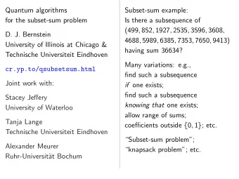
Quantum algorithms for the subset-sum problem D. J. Bernstein University of Illinois at Chicago & Technische Universiteit Eindhoven Joint work with: Stacey Jeffery University of Waterloo Tanja Lange Technische Universiteit Eindhoven Alexander Meurer Ruhr-Universit¨ at Bochum

Subset-sum example: Is there a subsequence of (499 ❀ 852 ❀ 1927 ❀ 2535 ❀ 3596 ❀ 3608 ❀ 4688 ❀ 5989 ❀ 6385 ❀ 7353 ❀ 7650 ❀ 9413) having sum 36634? Many variations: e.g., find such a subsequence if one exists; find such a subsequence knowing that one exists; allow range of sums; coefficients outside ❢ 0 ❀ 1 ❣ ; etc. “Subset-sum problem”; “knapsack problem”; etc.

The lattice connection Define ① 1 = 499, ✿ ✿ ✿ , ① 12 = 9413. Define ▲ ✒ Z 12 as ❢ ✈ : ✈ 1 ① 1 + ✁ ✁ ✁ + ✈ 12 ① 12 = 0 ❣ . Define ✉ ✷ Z 12 as (70 ❀ 2 ❀ 0 ❀ 0 ❀ 0 ❀ 0 ❀ 0 ❀ 0 ❀ 0 ❀ 0 ❀ 0 ❀ 0). If ❏ ✒ ❢ 1 ❀ 2 ❀ ✿ ✿ ✿ ❀ 12 ❣ and P ✐ ✷ ❏ ① ✐ = 36634 then ✈ ✷ ▲ where ✈ ✐ = ✉ ✐ � [ ✐ ✷ ❏ ]. ✈ is very close to ✉ . Reasonable to hope that ✈ is the closest vector in ▲ to ✉ . Subset-sum algorithms ✙ codimension-1 CVP algorithms.

The coding connection A weight- ✇ subset-sum problem: Is there a subsequence of (499 ❀ 852 ❀ 1927 ❀ 2535 ❀ 3596 ❀ 3608 ❀ 4688 ❀ 5989 ❀ 6385 ❀ 7353 ❀ 7650 ❀ 9413) having length ✇ and sum 36634?

The coding connection A weight- ✇ subset-sum problem: Is there a subsequence of (499 ❀ 852 ❀ 1927 ❀ 2535 ❀ 3596 ❀ 3608 ❀ 4688 ❀ 5989 ❀ 6385 ❀ 7353 ❀ 7650 ❀ 9413) having length ✇ and sum 36634? Replace Z with ( Z ❂ 2) ♠ : Is there a subsequence of (499 ❀ 852 ❀ 1927 ❀ 2535 ❀ 3596 ❀ 3608 ❀ 4688 ❀ 5989 ❀ 6385 ❀ 7353 ❀ 7650 ❀ 9413) having length ✇ and xor 1060? This is the central algorithmic problem in coding theory.

Recent asymptotic news Eurocrypt 2010 Howgrave-Graham–Joux: subset-sum exponent ✙ 0 ✿ 337. (Incorrect claim: ✙ 0 ✿ 311.) Eurocrypt 2011 Becker–Coron–Joux: subset-sum exponent ✙ 0 ✿ 291. Adaptations to decoding: Asiacrypt 2011 May–Meurer– Thomae, Eurocrypt 2012 Becker–Joux–May–Meurer.

Post-quantum subset sum Claimed in TCC 2010 Lyubashevsky–Palacio–Segev “Public-key cryptographic primitives provably as secure as subset sum”: There are “currently no known quantum algorithms that perform better than classical ones on the subset sum problem”. Hmmm. What’s the best quantum subset-sum exponent?

Quantum search (0.5) Assume that function ❢ has ♥ -bit input, unique root. Generic brute-force search finds this root using ✙ 2 ♥ evaluations of ❢ . 1996 Grover method finds this root using ✙ 2 0 ✿ 5 ♥ quantum evaluations of ❢ on superpositions of inputs. Cost of quantum evaluation of ❢ ✙ cost of evaluation of ❢ if cost counts qubit “operations”.

Easily adapt to handle different # of roots, and # not known in advance. Faster if # is large, but typically # is not very large. Most interesting: # ✷ ❢ 0 ❀ 1 ❣ .

Easily adapt to handle different # of roots, and # not known in advance. Faster if # is large, but typically # is not very large. Most interesting: # ✷ ❢ 0 ❀ 1 ❣ . Apply to the function ❏ ✼✦ Σ( ❏ ) � t where Σ( ❏ ) = P ✐ ✷ ❏ ① ✐ . Cost 2 0 ✿ 5 ♥ to find root (i.e., to find indices of subsequence of ① 1 ❀ ✿ ✿ ✿ ❀ ① ♥ with sum t ) or to decide that no root exists. We suppress poly factors in cost.

Algorithm details for unique root: Represent ❏ ✒ ❢ 1 ❀ ✿ ✿ ✿ ❀ ♥ ❣ as an integer between 0 and 2 ♥ � 1. ♥ bits are enough space to store one such integer. ♥ qubits store much more, a superposition over sets ❏ : 2 ♥ complex amplitudes ❛ 0 ❀ ✿ ✿ ✿ ❀ ❛ 2 ♥ � 1 with ❥ ❛ 0 ❥ 2 + ✁ ✁ ✁ + ❥ ❛ 2 ♥ � 1 ❥ 2 = 1. Measuring these ♥ qubits has chance ❥ ❛ ❏ ❥ 2 to produce ❏ . Start from uniform superposition, i.e., ❛ ❏ = 1 ❂ 2 ♥❂ 2 for all ❏ .

Step 1: Set ❛ ✥ ❜ where ❜ ❏ = � ❛ ❏ if Σ( ❏ ) = t , ❜ ❏ = ❛ ❏ otherwise. This is about as easy as computing Σ. Step 2: “Grover diffusion”. Set ❛ ✥ ❜ where ❜ ❏ = � ❛ ❏ + (2 ❂ 2 ♥ ) P ■ ❛ ■ . This is also easy. Repeat steps 1 and 2 about 0 ✿ 58 ✁ 2 0 ✿ 5 ♥ times. Measure the ♥ qubits. With high probability this finds the unique ❏ such that Σ( ❏ ) = t .

Graph of ❏ ✼✦ ❛ ❏ for 36634 example with ♥ = 12 after 0 steps: 1.0 0.5 0.0 −0.5 −1.0

Graph of ❏ ✼✦ ❛ ❏ for 36634 example with ♥ = 12 after Step 1: 1.0 0.5 0.0 −0.5 −1.0

Graph of ❏ ✼✦ ❛ ❏ for 36634 example with ♥ = 12 after Step 1 + Step 2: 1.0 0.5 0.0 −0.5 −1.0

Graph of ❏ ✼✦ ❛ ❏ for 36634 example with ♥ = 12 after Step 1 + Step 2 + Step 1: 1.0 0.5 0.0 −0.5 −1.0

Graph of ❏ ✼✦ ❛ ❏ for 36634 example with ♥ = 12 after 2 ✂ (Step 1 + Step 2): 1.0 0.5 0.0 −0.5 −1.0

Graph of ❏ ✼✦ ❛ ❏ for 36634 example with ♥ = 12 after 3 ✂ (Step 1 + Step 2): 1.0 0.5 0.0 −0.5 −1.0

Graph of ❏ ✼✦ ❛ ❏ for 36634 example with ♥ = 12 after 4 ✂ (Step 1 + Step 2): 1.0 0.5 0.0 −0.5 −1.0

Graph of ❏ ✼✦ ❛ ❏ for 36634 example with ♥ = 12 after 5 ✂ (Step 1 + Step 2): 1.0 0.5 0.0 −0.5 −1.0

Graph of ❏ ✼✦ ❛ ❏ for 36634 example with ♥ = 12 after 6 ✂ (Step 1 + Step 2): 1.0 0.5 0.0 −0.5 −1.0

Graph of ❏ ✼✦ ❛ ❏ for 36634 example with ♥ = 12 after 7 ✂ (Step 1 + Step 2): 1.0 0.5 0.0 −0.5 −1.0

Graph of ❏ ✼✦ ❛ ❏ for 36634 example with ♥ = 12 after 8 ✂ (Step 1 + Step 2): 1.0 0.5 0.0 −0.5 −1.0

Graph of ❏ ✼✦ ❛ ❏ for 36634 example with ♥ = 12 after 9 ✂ (Step 1 + Step 2): 1.0 0.5 0.0 −0.5 −1.0

Graph of ❏ ✼✦ ❛ ❏ for 36634 example with ♥ = 12 after 10 ✂ (Step 1 + Step 2): 1.0 0.5 0.0 −0.5 −1.0

Graph of ❏ ✼✦ ❛ ❏ for 36634 example with ♥ = 12 after 11 ✂ (Step 1 + Step 2): 1.0 0.5 0.0 −0.5 −1.0

Graph of ❏ ✼✦ ❛ ❏ for 36634 example with ♥ = 12 after 12 ✂ (Step 1 + Step 2): 1.0 0.5 0.0 −0.5 −1.0

Graph of ❏ ✼✦ ❛ ❏ for 36634 example with ♥ = 12 after 13 ✂ (Step 1 + Step 2): 1.0 0.5 0.0 −0.5 −1.0

Graph of ❏ ✼✦ ❛ ❏ for 36634 example with ♥ = 12 after 14 ✂ (Step 1 + Step 2): 1.0 0.5 0.0 −0.5 −1.0

Graph of ❏ ✼✦ ❛ ❏ for 36634 example with ♥ = 12 after 15 ✂ (Step 1 + Step 2): 1.0 0.5 0.0 −0.5 −1.0

Graph of ❏ ✼✦ ❛ ❏ for 36634 example with ♥ = 12 after 16 ✂ (Step 1 + Step 2): 1.0 0.5 0.0 −0.5 −1.0

Graph of ❏ ✼✦ ❛ ❏ for 36634 example with ♥ = 12 after 17 ✂ (Step 1 + Step 2): 1.0 0.5 0.0 −0.5 −1.0

Graph of ❏ ✼✦ ❛ ❏ for 36634 example with ♥ = 12 after 18 ✂ (Step 1 + Step 2): 1.0 0.5 0.0 −0.5 −1.0

Graph of ❏ ✼✦ ❛ ❏ for 36634 example with ♥ = 12 after 19 ✂ (Step 1 + Step 2): 1.0 0.5 0.0 −0.5 −1.0

Graph of ❏ ✼✦ ❛ ❏ for 36634 example with ♥ = 12 after 20 ✂ (Step 1 + Step 2): 1.0 0.5 0.0 −0.5 −1.0

Graph of ❏ ✼✦ ❛ ❏ for 36634 example with ♥ = 12 after 25 ✂ (Step 1 + Step 2): 1.0 0.5 0.0 −0.5 −1.0

Graph of ❏ ✼✦ ❛ ❏ for 36634 example with ♥ = 12 after 30 ✂ (Step 1 + Step 2): 1.0 0.5 0.0 −0.5 −1.0

Graph of ❏ ✼✦ ❛ ❏ for 36634 example with ♥ = 12 after 35 ✂ (Step 1 + Step 2): 1.0 0.5 0.0 −0.5 −1.0 Good moment to stop, measure.

Graph of ❏ ✼✦ ❛ ❏ for 36634 example with ♥ = 12 after 40 ✂ (Step 1 + Step 2): 1.0 0.5 0.0 −0.5 −1.0

Graph of ❏ ✼✦ ❛ ❏ for 36634 example with ♥ = 12 after 45 ✂ (Step 1 + Step 2): 1.0 0.5 0.0 −0.5 −1.0

Graph of ❏ ✼✦ ❛ ❏ for 36634 example with ♥ = 12 after 50 ✂ (Step 1 + Step 2): 1.0 0.5 0.0 −0.5 −1.0 Traditional stopping point.

Graph of ❏ ✼✦ ❛ ❏ for 36634 example with ♥ = 12 after 60 ✂ (Step 1 + Step 2): 1.0 0.5 0.0 −0.5 −1.0

Graph of ❏ ✼✦ ❛ ❏ for 36634 example with ♥ = 12 after 70 ✂ (Step 1 + Step 2): 1.0 0.5 0.0 −0.5 −1.0

Graph of ❏ ✼✦ ❛ ❏ for 36634 example with ♥ = 12 after 80 ✂ (Step 1 + Step 2): 1.0 0.5 0.0 −0.5 −1.0

Graph of ❏ ✼✦ ❛ ❏ for 36634 example with ♥ = 12 after 90 ✂ (Step 1 + Step 2): 1.0 0.5 0.0 −0.5 −1.0

Graph of ❏ ✼✦ ❛ ❏ for 36634 example with ♥ = 12 after 100 ✂ (Step 1 + Step 2): 1.0 0.5 0.0 −0.5 −1.0 Very bad stopping point.

❏ ✼✦ ❛ ❏ is completely described by a vector of two numbers (with fixed multiplicities): (1) ❛ ❏ for roots ❏ ; (2) ❛ ❏ for non-roots ❏ . Step 1 + Step 2 act linearly on this vector. Easily compute eigenvalues and powers of this linear map to understand evolution of state of Grover’s algorithm. ✮ Probability is ✙ 1 after ✙ ( ✙❂ 4)2 0 ✿ 5 ♥ iterations.