Quantile Regression for Large-scale Applications Jiyan Yang - PowerPoint PPT Presentation

Quantile Regression for Large-scale Applications Jiyan Yang Stanford University June 19, 2013 International Conference on Machine Learning, 2013 Joint work with Xiangrui Meng and Michael Mahoney Jiyan Yang (Stanford University) 2013 ICML June 19, 2013 1 / 27

Overview to quantile regression 1 Technical ingredients 2 Important notions Sampling lemma Conditioning Estimating row norms Main algorithm 3 Empirical evaluation 4 Medium-scale Empirical evaluation Large-scale Empirical evaluation Conclusion 5 Jiyan Yang (Stanford University) 2013 ICML June 19, 2013 2 / 27

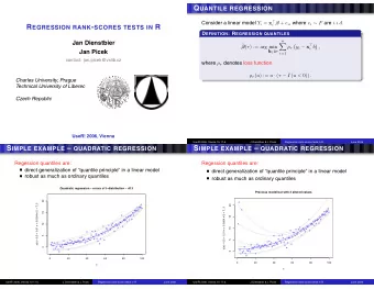
Overview to quantile regression What is quantile regression? Quantile regression is a method to estimate the quantiles of the conditional distribution of response. Quantile regression involves minimizing asymmetrically weighted absolute residuals: � τ z , z ≥ 0; ρ τ ( z ) = ( τ − 1) z , z < 0 . ℓ 1 regression is a special case of quantile regression with τ = 0 . 5. τ = 0.75 τ = 0.5 0.8 0.5 0.4 0.6 0.3 0.4 0.2 0.2 0.1 0 0 −1 −0.5 0 0.5 1 −1 −0.5 0 0.5 1 Jiyan Yang (Stanford University) 2013 ICML June 19, 2013 3 / 27

Overview to quantile regression Formulation of quantile regression Given matrix A ∈ R n × d , a vector b ∈ R n , and a parameter τ ∈ (0 , 1), quantile regression problem can be solved via the optimization problem minimize x ∈ R d ρ τ ( Ax − b ) , (1) where ρ τ ( y ) = � n i =1 ρ τ ( y i ), for y ∈ R n . � � We use A to denote − b , the quantile regression problem (1) A can equivalently be expressed as the following, minimize x ∈C ρ τ ( Ax ) , (2) where C = { x ∈ R d | c T x = 1 } and c is a unit vector with the last coordinate 1. Goal: For A ∈ R n × d with n ≫ d , find ˆ x such that x ) ≤ (1 + ǫ ) ρ τ ( Ax ∗ ) , ρ τ ( A ˆ where x ∗ is an optimal solution. Jiyan Yang (Stanford University) 2013 ICML June 19, 2013 4 / 27

Overview to quantile regression Background The standard solver for quantile regression problem is interior-point method ipm [Portnoy and Koenker, 1997], which might be applicable for medium-large scale problem with size 1 e 6 by 50. The best previous sampling algorithm, namely prqfn , for quantile regression problems is using an interior-point method on a smaller problem that has been preprocessed by randomly sampling a subset of the data; see [Portnoy and Koenker, 1997]. Inspired by recent work using randomized algorithms to compute approximate solutions for least-squares regression and related problems. For example, [Dasgupta et al., 2009] and [Clarkson et al., 2013]. Jiyan Yang (Stanford University) 2013 ICML June 19, 2013 5 / 27

Overview to quantile regression Comparison of three types of regression problems ℓ 2 regression ℓ 1 regression quantile regression estimation mean median quantile τ x 2 loss function | x | ρ τ ( x ) � Ax − b � 2 formulation � Ax − b � 1 ρ τ ( Ax − b ) 2 is a norm? yes yes no L 2 regression L 1 regression Quantile regression 1 0.8 0.4 0.6 0.3 0.5 0.4 0.2 0.2 0.1 0 0 0 −1 0 1 −1 0 1 −1 0 1 Jiyan Yang (Stanford University) 2013 ICML June 19, 2013 6 / 27

Technical ingredients Important notions Two important notions Definition (( α, β )-conditioning and well-conditioned basis (Dasgupta et al., 2009)) Given A ∈ R n × d , A is ( α, β )-conditioned if � A � 1 ≤ α and for all x ∈ R d , β � Ax � 1 ≥ � x � ∞ . Define κ ( A ) as the minimum value of αβ such that A is ( α, β )-conditioned. We will say that a basis U of range( A ) is a well-conditioned basis if κ = κ ( U ) is a low-degree polynomial in d , independent of n . Definition ( ℓ 1 leverage scores (Clarkson et al., 2013)) Given a well-conditioned basis U for the range( A ), the leverage scores of A are defined by the ℓ 1 norms of U ’s rows: � U ( i ) � 1 , i = 1 , . . . , n . Jiyan Yang (Stanford University) 2013 ICML June 19, 2013 7 / 27

Technical ingredients Important notions A useful tool Definition ((1 ± ǫ )-distortion Subspace-preserving Embedding) Given A ∈ R n × d , S ∈ R s × n is a (1 ± ǫ )-distortion subspace-preserving matrix if s = poly( d ) and for all x ∈ R d , (1 − ǫ ) ρ τ ( Ax ) ≤ ρ τ ( SAx ) ≤ (1 + ǫ ) ρ τ ( Ax ) . (3) Solving the subproblem min x ∈C ρ τ ( SAx ) gives a (1 + ǫ ) / (1 − ǫ )-approximate solution to the original problem. This is because 1 1 − ερ τ ( SAx ∗ ) ≤ 1 + ε 1 1 − ερ τ ( Ax ∗ ) . ρ τ ( A ˆ x ) ≤ 1 − ερ τ ( SA ˆ x ) ≤ Jiyan Yang (Stanford University) 2013 ICML June 19, 2013 8 / 27

Technical ingredients Sampling lemma Sampling lemma Lemma (Subspace-preserving Sampling Lemma) Given A ∈ R n × d , let U ∈ R n × d be a well-conditioned basis for range ( A ) with condition number κ . For s > 0 , choose ˆ p i ≥ min { 1 , s · � U ( i ) � 1 / � U � 1 } , and let S ∈ R n × n be a random diagonal matrix with S ii = 1 / ˆ p i with probability ˆ p i , and 0 otherwise. Then when ǫ < 1 / 2 and � � � � 4 �� τ 27 κ τ 18 s ≥ d log + log , (4) ǫ 2 1 − τ 1 − τ ǫ δ with probability at least 1 − δ , for every x ∈ R d , (1 − ε ) ρ τ ( Ax ) ≤ ρ τ ( SAx ) ≤ (1 + ε ) ρ τ ( Ax ) . Jiyan Yang (Stanford University) 2013 ICML June 19, 2013 9 / 27

Technical ingredients Sampling lemma Strategy Find a well-conditioned basis U . Compute or estimate the ℓ 1 row norms of U and construct sampling matrix S . Solve the subproblem minimize x ∈C ρ τ ( SAx ). Jiyan Yang (Stanford University) 2013 ICML June 19, 2013 10 / 27

Technical ingredients Conditioning Conditioning We call the procedure for finding U as conditioning. There are many existing conditioning methods. See [Clarkson et al., 2013] and [Dasgupta et al., 2009]. We care about two important properties: the condition number κ of the resulting basis U and the running time for construction. In general, there is a trade-off between these two quantities. Jiyan Yang (Stanford University) 2013 ICML June 19, 2013 11 / 27

Technical ingredients Conditioning Comparison of conditioning methods name running time type κ O ( nd 2 log d ) O ( d 5 / 2 log 3 / 2 n ) SC[SW11] QR O ( d 7 / 2 log 5 / 2 n ) FC [CDMMMW13] O ( nd log d ) QR O ( nd 5 log n ) d 3 / 2 ( d + 1) 1 / 2 Ellipsoid rounding [Cla05] ER O ( nd 3 log n ) 2 d 2 Fast ER [CDMMMW13] ER 13 11 SPC1 [MM13] O (nnz( A )) O ( d 2 log 2 d ) QR 6 d 2 SPC2 [MM13] O (nnz( A ) · log( n )) + ER small QR+ER 19 11 4 log 4 d ) SPC3 (this work) O (nnz( A ) · log( n )) + QR small O ( d QR+QR Table: Summary of running time, condition number, and type of conditioning methods proposed recently. QR and ER refer, respectively, to methods based on the QR factorization and methods based on Ellipsoid Rounding. SC := Slow Cauchy Transform FC := Fast Cauchy Transform SPC := Sparse Cauchy Transform Jiyan Yang (Stanford University) 2013 ICML June 19, 2013 12 / 27

Technical ingredients Estimating row norms Estimating row norms of well-conditioned basis Recall, that we choose our sampling probabilities based on the ℓ 1 row norms of a well-conditioned basis: ˆ p i ≥ min { 1 , s · � U ( i ) � 1 / � U � 1 } . Generally, we find a matrix R such that AR − 1 is a well-conditioned basis. We post-multiply a random projection matrix Π ∈ R d ×O (log n ) on AR − 1 and compute the median of each row of the resulting matrix. This gives us an estimation of the ℓ 1 row norms of AR − 1 up to some constant factor running in O (nnz( A ) · log n ) time; see [Clarkson et al., 2013]. R − 1 A Π          ·  ·       Jiyan Yang (Stanford University) 2013 ICML June 19, 2013 13 / 27

Main algorithm Fast Randomized Algorithm for Quantile Regression Input: A ∈ R n × d with full column rank, ǫ ∈ (0 , 1 / 2), τ ∈ [1 / 2 , 1). x ∈ R d to problem minimize x ∈C ρ τ ( Ax ). Output: An approximate solution ˆ 1: Compute R ∈ R d × d such that AR − 1 is a well-conditioned basis for range( A ). 2: Compute a (1 ± ǫ )-distortion subspace-preserving embedding S ∈ R s × n . x ∈ R d that minimizes ρ τ ( SAx ) with respect to x ∈ C . 3: Return ˆ Theorem (Fast Quantile Regression) Given A ∈ R n × d and ε ∈ (0 , 1 / 2) , the above algorithm returns a vector ˆ x that, with probability at least 0.8, satisfies � 1 + ε � ρ τ ( Ax ∗ ) , ρ τ ( A ˆ x ) ≤ 1 − ε where x ∗ is an optimal solution to the original problem. In addition, the algorithm to construct ˆ x runs in time O ( µ d 3 log( µ/ǫ ) /ǫ 2 ) , d � � O (nnz( A ) · log n ) + φ , (5) τ where µ = 1 − τ and φ ( s , d ) is the time to solve a quantile regression problem of size s × d. Jiyan Yang (Stanford University) 2013 ICML June 19, 2013 14 / 27

Empirical evaluation Outline of empirical evaluation We will show numerical results for medium-scale data with size about 1 e 6 by 50 as well as large-scale data with size 1 . 1 e 10 by 10; plots of relative errors versus sampling size, lower dimension and so on by using different conditioning-based methods; comparison of running time performance with existed methods. Jiyan Yang (Stanford University) 2013 ICML June 19, 2013 15 / 27