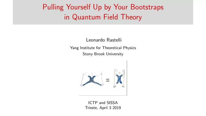

Pulling Yourself Up by Your Bootstraps in Quantum Field Theory Leonardo Rastelli Yang Institute for Theoretical Physics Stony Brook University ICTP and SISSA Trieste, April 3 2019
Quantum Field Theory in Fundamental Physics Local quantum fields { ϕ i ( x ) } x = ( t, � x ) , with t = time, � x = space The language of particle physics: for each particle species, a field
Quantum Field Theory for Collective Behavior Modelling N → ∞ degrees of freedom in statistical mechanics. Example: Ising model (uniaxial ferromagnet) σ i = ± 1 , spin at lattice site i Energy H = − J � ( ij ) σ i σ j Near T c , field theory description: magnetization ϕ ( � x ) ∼ � σ ( � x ) � , � � ∇ ϕ + m 2 ϕ 2 + λ ϕ 4 + . . . � ∇ ϕ · � � d 3 x H = m 2 ∼ T − T c
� � ∇ ϕ + m 2 ϕ 2 + λ ϕ 4 + . . . � ∇ ϕ · � � d 3 x H = The dots stand for higher-order “operators”: ϕ 6 , ( � ∇ ϕ · � ∇ ϕ ) ϕ 2 , ϕ 8 , etc. They are irrelevant for the large-distance physics at T ∼ T c . Crude rule of thumb: an operator O is irrelevant if its scaling weight [ O ] > 3 ( 3 ≡ d , dimension of space). Basic assignments: [ ϕ ] = 1 ⇒ [ � 2 ≡ d 2 − 1 and [ � x ] = − 1 = ∇ ] = 1 . So [ ϕ 2 ] = 1 , [ ϕ 4 ] = 2 , [ � ∇ ϕ · � ∇ ϕ ] =3, while [ ϕ 8 ] = 4 etc. First hint of universality: critical exponents do not depend on details. E.g., C T ∼ | T − T c | − α , � ϕ � ∼ ( T c − T ) β for T < T c , etc.
QFT ≡ “Theory of fluctuating fields” (Duh!) Traditionally, QFT is formulated as a theory of local “quantum fields”: � � dϕ ( x ) e − H [ ϕ ( x )] Z = g x In particle physics, x ∈ space time and g = � (quantum) In statistical mechanics, x ∈ space and g = T (thermal). Difficult to calculate when g is not small.
Inadequacy of traditional viewpoint More conceptually , indications that a better framework is needed: Theories with no H [ ϕ ( x )] . g ′ = 1 T [ ϕ ; g ] ⇔ T ′ [ ϕ ′ ; g ′ ] , g Paradigm: 6 d (2 , 0) theory. T [ ϕ ; g ] M5 { N T ′ [ ϕ ′ ; g ′ ]
Our vision: the Bootstrap Determining Theory Space using Consistency: Symmetries & Quantum Mechanics. Sharp rigorous predictions without resorting to approximations. Ultimate goal: compile a complete catalogue of consistent QFTs. [Wikipedia: Bootstrap is “a self-starting process that is supposed to proceed without external input” ]
A picture of Theory Space Height = a measure of the number of degrees of freedom. Stationary points = Theories that look the same at all length scales, called Conformal Field Theories. They are defined by an abstract operator algebra. We “flow” from higher to lower points by “integrating out” short-distance d.o.f. This can be made rigorous in d = 2 : the “height” is called the c -function.
Scale → Conformal Physics simplifies when intrinsic length scales can be neglected: high/low energy regimes of QFTs and statistical systems near T c . Scale invariance is “generically” enhanced to conformal invariance. A conformal transformation acts locally as rotation and dilatation.
Abstract Conformal Field Theory A CFT is defined by the correlations �O 1 ( x 1 ) . . . O n ( x n ) � of local operators {O k ( x ) } . E.g., in Ising CFT we have: the spin operator σ ( x ) , the energy operator ǫ ( x ) , and infinitely many more. Scaling dimensions ∆ i : �O i ( x ) O i ( y ) � = | x − y | − 2∆ i , related to critical exponents, e.g. , α = 3 − 2∆ ǫ 3 − ∆ ǫ . Operator Product Expansion c ijk | x − y | ∆ k − ∆ i − ∆ j ( O k ( y ) + . . . ) . � OPE : O i ( x ) O j ( y ) = k The sum converges (unlike in a general QFT).
Conformal bootstrap The data { ∆ i , c ijk } determine the theory. Old aspiration (1970s) Polyakov, Ferrara Gatto Grillo: Impose crossing symmetry to solve for these data. For a 4-point function:
“Madamina, il catalogo ` e questo: ...ma in Ispagna son gi` a mille e tre” Famous success story in d = 2 . Conformal symmetry is infinite dimensional. In some cases, only finite number of independent O i ⇒ exact solution of the bootstrap. Complete catalogue of (unitary) CFTs M p with c < 1 . Labelled by an integer p ≥ 3 , with 6 c = 1 − p ( p + 1) ◮ p = 3 , c = 1 / 2 , Ising model. ◮ p = 4 , c = 7 / 10 , tricritical Ising model. ◮ p = 5 , c = 4 / 5 , three-state Potts model. ◮ . . .
The modern bootstrap program Rattazzi Rychkov Tonni Vichi, 2008 Crossing + positive probability ⇒ inequalities for { ∆ i , c ijk } . Bootstrap inequalities obtained numerically but perfectly rigorous: they may not be optimal but they are true.
Bootstrap of 3 d Ising CFT El-Showk Paulos Poland Rychkov Simmons-Duffin Vichi, Kos Poland S-D CFT in d = 3 with up/down symmetry. σ odd, ǫ even, σ × σ = 1 + ǫ + . . . Assuming that σ , ǫ are the only relevant operators ( ∆ < 3 ) allowed region with ∆ σ ′ ≥ 3 ( n max = 6) ∆ � 1 . 7 1 . 6 1 . 5 1 . 4 1 . 3 1 . 2 1 . 1 ∆ σ 1 0 . 5 0 . 51 0 . 52 0 . 53 0 . 54 0 . 55 0 . 56 0 . 57 0 . 58 3 d Ising gets cornered. Critical universality explained! Most precise determination of critical exponents. Rigorous error bars.
Charting Theory Space The modern bootstrap is a very flexible tool: works for any dimension, any symmetry. ◮ The CFT genome project: Find the list of CFTs with a small number of relevant operators. Some partial results. Adding symmetries makes theories more rigid and more tractable. Supersymmetry (fermions ↔ bosons) is a theorist’s favorite. SuperCFTs play a central role in modern physical mathematics. ◮ Full classification program for superCFTs. They exist only for d ≤ 6 (Nahm ’77). Classification facilated by solvable subsectors identical to well-studied mathematical structures, such as vertex operator algebras.
The Great Mother: The Six-dimensional (2 , 0) Theory (2 , 0) N theory governs low-energy M5 fluctuations of N five-branes in M-theory, a quantum gravity theory in 11 dimensions { N ◮ Maximally (super)symmetric QFT in highest dimension. ◮ Paradigm of a theory with no H [ ϕ ] . For fixed N , intrinsically quantum. Surprising that an interacting field theory exists at all in d = 6 . E.g., [ ϕ ] = 2 so [ ϕ 4 ] = 8 > d . No obvious microscopic description. ◮ “Mother” of huge landscape of QFTs in d < 6 , by compactification.
S 4 (2 , 0) N →∞ ∼ = 11d supergravity on AdS 7 Canonical holographic duality: Local CFT in flat space ≡ quantum gravity theory in Anti-de Sitter, in one higher dim. For large N , bulk side is weakly coupled: classical 11 d supergravity. CFT correlators = supergravity “scattering amplitudes” in AdS. They are entirely fixed by symmetry LR Zhou
Bootstrap of (2 , 0) N Theory Beem Lemos LR van Rees Minimal physical input: ∃ a tower of O BPS with ∆ = 4 , 6 , . . . 2 N . ∆ ( ∆ = conformal dimension) ◮ Bootstrap is solvable for a subalgebra {O χ } ⊃ {O BPS } ! Protected subalgebra {O χ } , with meromorphic correlators �O χ z 1 ) O χ z 2 ) . . . O χ 1 ( z 1 , ¯ 2 ( z 2 , ¯ n ( z n , ¯ z n ) � = f ( z i ) . Isomorphic to the left-moving sector of a 2 d CFT (= vertex operator algebra). (2 , 0) N → well-known W N algebra! Infinite dimensional symmetry. Exact 3-point functions of for any N . For N → ∞ , striking agreement with supergravity on AdS 7 × S 4 . One recovers non-linear supergravity purely from algebraic consistency. 1 /N corrections ⇒ quantum M-theory corrections.
◮ For “non-protected” operators (non-integer ∆ ), numerical bootstrap. For N = 2 , strong evidence that bootstrap has unique solution! Conjecturally true for all N , using more complicated correlators. A blueprint for defining and solving the (2 , 0) N theory.
4d N = 2 SCFT − → 2d Chiral Algebra Any 4 d N = 2 SCFT has a protected subsector isomorphic to a 2 d chiral algebra ( aka a Vertex Operator Algebra). Beem Lemos Liendo Peelaers LR ◮ Always a Virasoro subalgebra with c 2 d = − 12 c 4 d c 4 d ≡ Weyl 2 conformal anomaly coefficient. ◮ Global flavor symmetry of SCFT → Affine Kac-Moody algebra ◮ Conjecture (Beem LR): Higgs branch ≡ associated variety of the VOA ◮ Supersymmetric index of the SCFT ≡ vacuum character χ ( q ) of the VOA Previous conjecture → χ ( q ) must obey a modular differential equation.
Some examples of VOAs from 4 d SCFTs ◮ SU (2) super QCD with N f = 4 ⇒ so (8) − 2 AKM algebra. ◮ E 6 SCFT ⇒ ( e 6 ) − 3 AKM algebra. ◮ N = 4 SYM ⇒ N = 4 super W -algebra, with generators given by chiral primaries of dimensions { h i = r i +1 2 } , { r i } ≡ exponents of gauge group G . ◮ ( A 1 , A 2 k ) Argyes-Douglas theories ⇒ Virasoro algebra of (2 , 2 k + 3) model
6 = 4 +2: class S (ix) theories Gaiotto Put (2 , 0) on R 4 × C . C ≡ Riemann surface with punctures. ⇓ N = 2 SUSY CFT on R 4 . Theory space as a real physical space, the surface C ! Consistency conditions in theory space. E.g., a TQFT valued in VOAs! Degeneration of C ⇒ Theory T [ C ] splits into decoupled theories. [Roy Sato’s drawing]
I’ve emphasized two heuristic principles: ◮ Enlarge the view to the whole space of QFTs. ◮ Bootstrap approach: Use internal consistency rules and symmetries to chart theory space, rather than solving detailed “microscopic” models. (From the Salt Lake Tribune)
Concrete models... As physicists, we often build detailed dynamical models: Identify relevant degrees of freedom { ϕ i } ↓ Write a model H [ ϕ i ] ↓ Solve it
Recommend
More recommend