Pseudo-Marginal Hamiltonian Monte Carlo with Efficient Importance - PowerPoint PPT Presentation
Pseudo-Marginal Hamiltonian Monte Carlo with Efficient Importance Sampling Kjartan Kloster Osmundsen 1 Tore Selland Kleppe 1 Roman Liesenfeld 2 1 Department of Mathematics and Physics University of Stavanger, Norway 2 Institute of Econometrics and
Pseudo-Marginal Hamiltonian Monte Carlo with Efficient Importance Sampling Kjartan Kloster Osmundsen 1 Tore Selland Kleppe 1 Roman Liesenfeld 2 1 Department of Mathematics and Physics University of Stavanger, Norway 2 Institute of Econometrics and Statistics University of Cologne, Germany EcoSta 2018 City University of Hong Kong 20th June 2018 Osmundsen, Kleppe, Liesenfeld Pseudo-Marginal HMC with EIS EcoSta 2018 1 / 12
Background and motivation Simulate from target distributions with strong nonlinear dependencies – Joint posterior of latent variables and parameters in Bayesian hierarchical models Current methods include: – Variants of Gibbs sampling (nonlinear dependencies across the blocks) – Jointly updating latent variables and parameters (need to ensure that proposals are properly aligned) – Pseudo-marginal methods Osmundsen, Kleppe, Liesenfeld Pseudo-Marginal HMC with EIS EcoSta 2018 2 / 12
Pseudo-marginal methods Target marginal posteriors of the parameters directly, by integrating out the latent variables Relies on ability to produce unbiased, low-variance Monte Carlo estimate of said posterior – Sequential Monte Carlo methods Our approach: Combining pseudo-marginal Hamiltonian Monte Carlo (Lindsten and Doucet, 2016) with Efficient Importance Sampling (Liesenfeld and Richard, 2003; Richard and Zhang, 2007) Osmundsen, Kleppe, Liesenfeld Pseudo-Marginal HMC with EIS EcoSta 2018 3 / 12
Hamiltonian Monte Carlo (HMC) General purpose MCMC method Energy preserving dynamical system as the proposal mechanism – Approximated by numerical integrator which preserves the dynamics Produces close to iid samples The main sampling algorithm in Stan, the popular Bayesian modeling software Osmundsen, Kleppe, Liesenfeld Pseudo-Marginal HMC with EIS EcoSta 2018 4 / 12
Pseudo-marginal HMC Directly targeting the marginal posterior p ( θ | y ) ∝ p ( θ ) p ( y | θ ) � p ( y | θ ) = p ( y | x , θ ) p ( x | θ ) d x is approximated numerically, using a set of random generated numbers u An augmented target distribution corrects for Monte Carlo variation: π ( θ , u ) ∝ p ( θ )ˆ ¯ p ( y | θ , u ) p ( u ) Regular HMC is applied to the augmented target The HMC integrator needs to evaluate ∇ ¯ π ( θ , u ), implemented using automatic differentiation software � To ensure good performance, p ( y | θ , u ) should be a smooth function of both u and θ – Typically not the case for sequential Monte Carlo methods Osmundsen, Kleppe, Liesenfeld Pseudo-Marginal HMC with EIS EcoSta 2018 5 / 12
Efficient Importance Sampling (EIS) � Our chosen algorithm for calculating p ( y | θ , u ) EIS chooses importance densities that minimizes the Monte Carlo variance of importance sampling estimates A suitable density class m ( x | ❛ , θ ) is chosen, where the EIS parameter ❛ is chosen so MCMC variance is minimized The local minimization problems for ❛ (one for each observation) are reduced to linear least squares problems, solved iteratively from a starting value ❛ 0 p ( y | x ( i ) , θ ) p ( x ( i ) | θ ) x ( i ) ∼ m ( ·| ❛ , θ , u ) � p ( y | θ , u ) = 1 � n , i =1 n m ( x ( i ) | ❛ , θ ) Osmundsen, Kleppe, Liesenfeld Pseudo-Marginal HMC with EIS EcoSta 2018 6 / 12
Simulation experiments State space models y t | x t , θ ∼ g t ( ·| x t , θ ) , t = 1 , . . . , T , x t | x t − 1 , θ ∼ N ( ·| µ t ( x t − 1 , θ ) , σ 2 t ( x t − 1 , θ )) , t = 2 , . . . , T , x 1 | θ ∼ N ( ·| µ 1 ( θ ) , σ 2 1 ( θ )) Stan is used as a benchmark Osmundsen, Kleppe, Liesenfeld Pseudo-Marginal HMC with EIS EcoSta 2018 7 / 12
One-parameter model y t ∼ exp( x t / 2) · ǫ t , ǫ t ∼ N (0 , 1) , t ∈ (1 , 2 , . . . , T ), x t ∼ θ + η t , η t ∼ N (0 , 1) , t ∈ (1 , 2 , . . . , T ) Simulated observations θ CPU time (s) Post. mean Post. std. ESS ESS/s HMC-EIS (0 reg) 16.4 0.026 0.063 631.8 38.4 HMC-EIS (1 reg) 74.2 0.026 0.063 876.5 11.8 Stan 2.1 0.026 0.063 319 151.2 Osmundsen, Kleppe, Liesenfeld Pseudo-Marginal HMC with EIS EcoSta 2018 8 / 12
Stochastic volatility model y t = exp( x t / 2) · ǫ t , ǫ t ∼ N (0 , 1) , t ∈ (1 , 2 , . . . , T ), x t = γ + δ x t − 1 + v η t , η t ∼ N (0 , 1) , t ∈ (2 , 3 , . . . , T ), γ v η 1 ∼ N (0 , 1) x 1 = 1 − δ + √ 1 − δ 2 η 1 , Dollar/Pound exchange rates δ CPU time (s) Post. mean Post. std. ESS ESS/s HMC-EIS (2 reg) 245 0.976 0.01 469 1.92 Stan 10 0.976 0.01 284 28.6 Osmundsen, Kleppe, Liesenfeld Pseudo-Marginal HMC with EIS EcoSta 2018 9 / 12
Constant elasticity of variance diffusion model ǫ t ∼ N (0 , 1) , t ∈ (1 , 2 , . . . , T ), y t = x t + σ y ǫ t , √ ∆ η t , x t = x t − 1 + ∆( α − β x t − 1 ) + σ x x γ t − 1 x 1 ∼ N ( y 1 , 0 . 01 2 ) , η t ∼ N (0 , 1) , t ∈ (2 , 3 , . . . , T ), Short-term interest rates Stan is not converging (limited information in the observations, σ y = 0 . 0005) – Compare our results to modified Cholesky Riemann manifold Hamiltonian Monte Carlo (MCRMHMC) and Particle Gibbs. α CPU time (s) Post. mean Post. std. ESS ESS/s HMC-EIS (1 reg) 473 0.01 0.009 1000 2.11 MCRMHMC 16200 0.01 0.009 1000 0.06 Particle Gibbs 90 0.01 0.009 456 5.07 σ x Post. mean Post. std. ESS ESS/s HMC-EIS (1 reg) 0.41 0.06 945 1.73 MCRMHMC 0.41 0.06 579 0.04 Particle Gibbs 0.41 0.06 79 0.88 Osmundsen, Kleppe, Liesenfeld Pseudo-Marginal HMC with EIS EcoSta 2018 10 / 12
Conclusion We have combined HMC with EIS Produces stable, effective and accurate results. Competitive computational cost for models with advanced latent processes. Osmundsen, Kleppe, Liesenfeld Pseudo-Marginal HMC with EIS EcoSta 2018 11 / 12
Thank you for your attention! Osmundsen, Kleppe, Liesenfeld Pseudo-Marginal HMC with EIS EcoSta 2018 12 / 12
Recommend
More recommend
Explore More Topics
Stay informed with curated content and fresh updates.


