Proximal Newton-type methods for minimizing composite functions - PowerPoint PPT Presentation

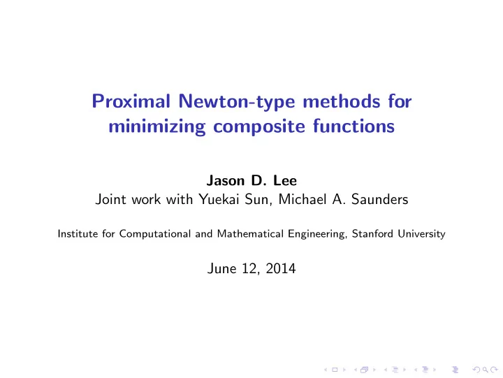
Proximal Newton-type methods for minimizing composite functions Jason D. Lee Joint work with Yuekai Sun, Michael A. Saunders Institute for Computational and Mathematical Engineering, Stanford University June 12, 2014

Minimizing composite functions Proximal Newton-type methods Inexact search directions Computational experiments

Minimizing composite functions minimize f ( x ) := g ( x ) + h ( x ) x ◮ g and h are convex functions ◮ g is continuously differentiable, and its gradient ∇ g is Lipschitz continuous ◮ h is not necessarily everywhere differentiable, but its proximal mapping can be evaluated efficiently

Minimizing composite functions: Examples ℓ 1 -regularized logistic regression: n 1 � log(1 + exp( − y i w T x i )) + λ � w � 1 . min n w ∈ R p i =1 Sparse inverse covariance: min − logdet (Θ) + tr ( S Θ) + λ � Θ � 1 Θ

Minimizing composite functions: Examples Graphical Model Structure Learning � � min − θ rj ( x r , x j ) + log Z ( θ ) + λ � θ rj � F . θ ( r,j ) ∈ E ( r,j ) ∈ E Multiclass Classification: � � n e w T yi x i � min − log + � W � ∗ � k e w T k x i W i =1

Minimizing composite functions: Examples Arbitrary convex program min g ( x ) + 1 C ( x ) x Equivalent to solving min x ∈ C g ( x )

The proximal mapping The proximal mapping of a convex function h is h ( y ) + 1 2 � y − x � 2 prox h ( x ) = arg min 2 . y ◮ prox h ( x ) exists and is unique for all x ∈ dom h ◮ proximal mappings generalize projections onto convex sets Example: soft-thresholding: Let h ( x ) = � x � 1 . Then prox t �·� 1 ( x ) = sign( x ) · max {| x | − t, 0 } .

The proximal gradient step x k +1 = prox t k h ( x k − t k ∇ g ( x k )) h ( y ) + 1 � y − ( x k − t k ∇ g ( x k )) � 2 = arg min 2 t k y = x k − t k G t k f ( x k ) ◮ G t k f ( x k ) minimizes a simple quadratic model of f : 1 ∇ g ( x k ) T d + � d � 2 − t k G t k f ( x k ) = arg min + h ( x k + d ) . 2 2 t k d � �� � simple quadratic ◮ G f ( x ) can be thought of as a generalized gradient of f ( x ) . Simplifies to the gradient descent on g ( x ) when h = 0 .

The proximal gradient method Algorithm 1 The proximal gradient method Require: starting point x 0 ∈ dom f 1: repeat Compute a proximal gradient step : 2: � � G t k f ( x k ) = 1 x k − prox t k h ( x k − t k ∇ g ( x k )) . t k Update: x k +1 ← x k − t k G t k f ( x k ) . 3: 4: until stopping conditions are satisfied.

Minimizing composite functions Proximal Newton-type methods Inexact search directions Computational experiments

Proximal Newton-type methods Main idea: use a local quadratic model (in lieu of a simple quadratic model) to account for the curvature of g : 1 ∇ g ( x k ) T d + 2 d T H k d ∆ x k := arg min + h ( x k + d ) . d � �� � local quadratic Solve the above subproblem and update x k +1 = x k + t k ∆ x k .

A generic proximal Newton-type method Algorithm 2 A generic proximal Newton-type method Require: starting point x 0 ∈ dom f 1: repeat Choose an approximation to the Hessian H k . 2: Solve the subproblem for a search direction: 3: ∆ x k ← arg min d ∇ g ( x k ) T d + 1 2 d T H k d + h ( x k + d ) . Select t k with a backtracking line search. 4: Update: x k +1 ← x k + t k ∆ x k . 5: 6: until stopping conditions are satisfied.

Why are these proximal? Definition (Scaled proximal mappings) Let h be a convex function and H , a positive definite matrix. Then the scaled proximal mapping of h at x is defined to be h ( y ) + 1 prox H 2 � y − x � 2 h ( x ) = arg min H . y The proximal Newton update is � � x k +1 = prox H k x k − H − 1 k ∇ g ( x k ) h and analogous to the proximal gradient update � � x k − 1 x k +1 = prox h/L L ∇ g ( x k ) ∆ x = 0 if and only if x minimizes f = g + h .

A classical idea Traces back to: ◮ Projected Newton-type methods ◮ Generalized proximal point methods Popular methods tailored to specific problems: ◮ glmnet : lasso and elastic-net regularized generalized linear models ◮ LIBLINEAR: ℓ 1 -regularized logistic regression ◮ QUIC: sparse inverse covariance estimation

Choosing an approximation to the Hessian 1. Proximal Newton method: use Hessian ∇ 2 g ( x k ) 2. Proximal quasi-Newton methods: build an approximation to ∇ 2 g ( x k ) using changes in ∇ g : H k +1 ( x k +1 − x k ) = ∇ g ( x k ) − ∇ g ( x k +1 ) 3. If problem is large, use limited memory versions of quasi-Newton updates (e.g. L-BFGS) 4. Diagonal+rank 1 approximation to the Hessian. Bottom line: Most strategies for choosing Hessian approximations Newton-type methods also work for proximal Newton-type methods

Theoretical results Take home message : The convergence of proximal Newton methods parallel those of the regular Newton Method. Global convergence: ◮ smallest eigenvalue of H k ’s bounded away from zero Quadratic convergence (prox-Newton method): ◮ Quadratic convergence: � x k − x ⋆ � 2 ≤ c 2 k or log log 1 ǫ iterations to achieve ǫ accuracy. ◮ Assumptions: g is strongly convex, and ∇ 2 g is Lipschitz continuous Superlinear convergence (prox-quasi-Newton methods): ◮ BFGS, SR1, and many other hessian approximations. Dennis-More condition � ( H k −∇ 2 g ( x ⋆ ) ) ( x k +1 − x k ) � 2 → 0 . � x k +1 − x k � 2 ◮ Superlinear convergence means it is faster than any linear rate. E.g. c k 2 converges superlinearly to 0 .

Questions so far? Any Questions?

Minimizing composite functions Proximal Newton-type methods Inexact search directions Computational experiments

Solving the subproblem ∇ g ( x k ) T d + 1 2 d T H k d + h ( x k + d ) ∆ x k = arg min d = arg min g k ( x k + d ) + h ( x k + d ) ˆ d Usually, we must use an iterative method to solve this subproblem. ◮ Use proximal gradient or coordinate descent on the subproblem. ◮ A gradient/coordinate descent iteration on the subproblem is much cheaper than a gradient iteration on the original function f , since it does not require a pass over the data. By solving the subproblem, we are more efficiently using a gradient evaluation than gradient descent. ◮ H k is commonly a L-BFGS approximation, so computing a gradient takes O ( Lp ) . A gradient of the original function takes O ( np ) . The subproblem is independent of n .

Inexact Newton-type methods Main idea: no need to solve the subproblem exactly only need a good enough search direction. ◮ We solve the subproblem approximately with an iterative method, terminating (sometimes very) early ◮ number of iterations may increase, but computational expense per iteration is smaller ◮ many practical implementations use inexact search directions

What makes a stopping condition good? We should solve the subproblem more precisely when: 1. x k is close to x ⋆ , since Newton’s method converges quadratically in this regime. 2. ˆ g k + h is a good approximation to f in the vicinity of x k (meaning H k has captured the curvature in g ), since minimizing the subproblem also minimizes f .

Early stopping conditions For regular Newton’s method the most common stopping condition is �∇ ˆ g k ( x k + ∆ x k ) � ≤ η k �∇ g ( x k ) � . Analogously, � � � � � G (ˆ g k + h ) /M ( x k + ∆ x k ) ≤ η k � G f/M ( x k ) � � � �� � � �� � optimality of subproblem solution optimality of x k Choose η k based on how well G ˆ g k + h approximates G f : � � � G (ˆ g k − 1 + h ) /M ( x k ) − G f/M ( x k ) � η k ∼ � � � G f/M ( x k − 1 ) � Reflects the Intuition: solve the subproblem more precisely when ◮ G f/M is small, so x k is close to optimum. ◮ G ˆ g + h − G f ≈ 0 , means that H k is accurately capturing the curvature of g .

Convergence of the inexact prox-Newton method ◮ Inexact proximal Newton method converges superlinearly for the previous choice of stopping criterion and η k . ◮ In practice, the stopping criterion works extremely well. It uses approximately the same number of iterations as solving the subproblem exactly, but spends much less time on each subproblem.

Minimizing composite functions Proximal Newton-type methods Inexact search directions Computational experiments

Sparse inverse covariance (Graphical Lasso) Sparse inverse covariance: min − logdet (Θ) + tr ( S Θ) + λ � Θ � 1 Θ ◮ S is a sample covariance, and estimates Σ the population covariance. p � ( x i − µ )( x i − µ ) T S = i =1 ◮ S is not of full rank since n < p , so S − 1 doesn’t exist. ◮ Graphical lasso is a good estimator of Σ − 1

Sparse inverse covariance estimation Figure: Proximal BFGS method with three subproblem stopping conditions (Estrogen dataset p = 682 ) 0 0 10 10 adaptive adaptive Relative suboptimality Relative suboptimality maxIter = 10 maxIter = 10 −2 −2 exact exact 10 10 −4 −4 10 10 −6 −6 10 10 0 5 10 15 20 25 0 5 10 15 20 Function evaluations Time (sec)

Sparse inverse covariance estimation Figure: Leukemia dataset p = 1255 0 0 10 10 adaptive adaptive Relative suboptimality Relative suboptimality maxIter = 10 maxIter = 10 −2 −2 exact exact 10 10 −4 −4 10 10 −6 −6 10 10 0 5 10 15 20 25 0 50 100 Function evaluations Time (sec)