Properties of Transpose Transpose has higher precedence than - - PDF document

3.2, 3.3 Inverting Matrices

• P. Danziger

Properties of Transpose

Transpose has higher precedence than multiplica- tion and addition, so ABT = A

• BT

and A + BT = A +

• BT

As opposed to the bracketed expressions (AB)T and (A + B)T Example 1 Let A =

• 1

2 1 2 5 2

• and B =
• 1

1 1 1

• .

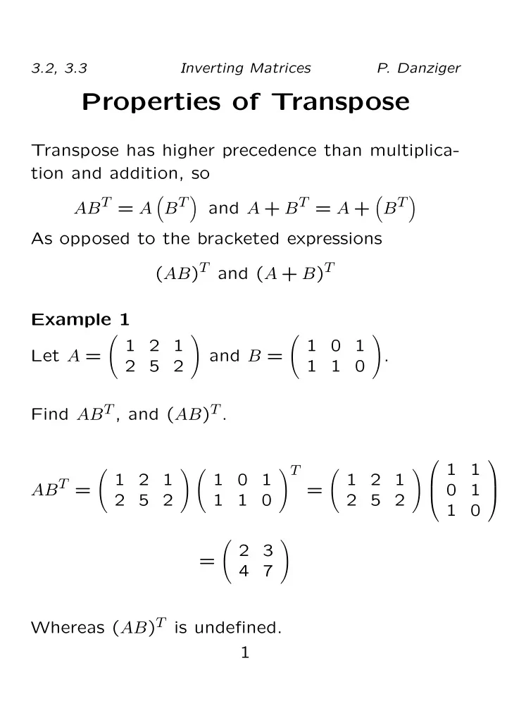
Find ABT, and (AB)T. ABT =

• 1

2 1 2 5 2 1 1 1 1

T

=

• 1

2 1 2 5 2

  

1 1 1 1

  

=

• 2

3 4 7

• Whereas (AB)T is undefined.

1

3.2, 3.3 Inverting Matrices

• P. Danziger

Theorem 2 (Properties of Transpose) Given ma- trices A and B so that the operations can be pre- formed

• 1. (AT)T = A
• 2. (A + B)T = AT + BT and (A − B)T = AT − BT
• 3. (kA)T = kAT
• 4. (AB)T = BTAT

2

3.2, 3.3 Inverting Matrices

• P. Danziger

Matrix Algebra

Theorem 3 (Algebraic Properties of Matrix Multiplication)

• 1. (k + ℓ)A = kA + ℓA (Distributivity of scalar

multiplication I)

• 2. k(A + B) = kA + kB (Distributivity of scalar

multiplication II)

• 3. A(B + C) = AB + AC (Distributivity of matrix

multiplication)

• 4. A(BC) = (AB)C (Associativity of matrix mul-

tiplication)

• 5. A + B = B + A (Commutativity of matrix ad-

dition)

• 6. (A + B) + C = A + (B + C) (Associativity of

matrix addition)

• 7. k(AB) = A(kB) (Commutativity of Scalar Mul-

tiplication) 3

3.2, 3.3 Inverting Matrices

• P. Danziger

The matrix 0 is the identity of matrix addition. That is, given a matrix A, A + 0 = 0 + A = A. Further 0A = A0 = 0, where 0 is the appropriately sized 0 matrix. Note that it is possible to have two non-zero ma- trices which multiply to 0. Example 4

• 1

−1 −1 1 1 1 1 1

• =
• 1 − 1

1 − 1 −1 + 1 −1 + 1

• =
• The matrix I is the identity of matrix multiplica-
• tion. That is, given an m × n matrix A,

AIn = ImA = A Theorem 5 If R is in reduced row echelon form then either R = I, or R has a row of zeros. 4

3.2, 3.3 Inverting Matrices

• P. Danziger

Theorem 6 (Power Laws) For any square ma- trix A, ArAs = Ar+s and (Ar)s = Ars Example 7 1.

  

1 1 1 2 2

  

4

=

      

1 1 1 2 2

  

2 

  

2

• 2. Find A6, where

A =

• 1

1 1

• A6 = A2A4 = A2

A22. Now A2 =

• 1

2 1

• , so

A2 A22 =

• 1

2 1 1 2 1

2

=

• 1

2 1 1 3 1

• =
• 1

5 1

• 5

3.2, 3.3 Inverting Matrices

• P. Danziger

Inverse of a matrix

Given a square matrix A, the inverse of A, denoted A−1, is defined to be the matrix such that AA−1 = A−1A = I Note that inverses are only defined for square ma- trices

Note Not all matrices have inverses.

If A has an inverse, it is called invertible. If A is not invertible it is called singular. 6

3.2, 3.3 Inverting Matrices

• P. Danziger

Example 8 1. A =

• 1

2 2 5

• A−1 =
• 5

−2 −2 1

• Check:
• 1

2 2 5 5 −2 −2 1

• =
• 1

1

• 2.

A =

• 1

2 2 4

• Has no inverse

3. A =

  

1 1 1 1 2 1 1 1 2

  

A−1 =

  

3 −1 −1 −1 1 −1 1

  

Check:

  

1 1 1 1 2 1 1 1 2

     

3 −1 −1 −1 1 −1 1

   =   

1 1 1

  

4. A =

  

1 2 1 2 1 3 3 3 4

  

Has no inverse 7

3.2, 3.3 Inverting Matrices

• P. Danziger

Inverses of 2 × 2 Matrices

Given a 2 × 2 matrix A =

• a

b c d

• A is invertible if and only if ad − bc = 0 and

A−1 = 1 ad − bc

• d

−b −c a

• The quantity ad − bc is called the determinant of

the matrix and is written det(A), or |A|. Example 9 A =

• 1

2 3 3

• A−1 =

1 −3

• 3

−2 −3 1

• =
• −1

2 3

1 −1

3

• Check:

1 −3

• 3

−2 −3 1 1 2 3 3

• = −1

3

• −3

−3

• = I

8

3.2, 3.3 Inverting Matrices

• P. Danziger

Algebra of Invertibility

Theorem 10 Given an invertible matrix A:

• 1. (A−1)−1 = A,
• 2. (An)−1 = (A−1)n
• = A−n

,

• 3. (kA)−1 = 1

kA−1,

• 4. (AT)−1 = (A−1)T,

9

3.2, 3.3 Inverting Matrices

• P. Danziger

Theorem 11 Given two invertible matrices A and B (AB)−1 = B−1A−1. Proof: Let A and B be invertible matricies and let C = AB, so C−1 = (AB)−1. Consider C = AB. Multiply both sides on the left by A−1: A−1C = A−1AB = B. Multiply both sides on the left by B−1. B−1A−1C = B−1B = I. So, B−1A−1 is the matrix you need to multiply C by to get the identity. Thus, by the definition of inverse B−1A−1 = C−1 = (AB)−1. 10

3.2, 3.3 Inverting Matrices

• P. Danziger

A Method for Inverses

Given a square matrix A and a vector b ∈ Rn, consider the equation Ax = b This represents a system of equations with coeffi- cient matrix A. Multiply both sides by A−1 on the left, to get A−1Ax = A−1b. But A−1A = In and Ix = x, so we have

x = A−1b.

Note that we have a unique solution. The as- sumption that A is invertible is equaivalent to the assumption that Ax = b has unique solution. 11

3.2, 3.3 Inverting Matrices

• P. Danziger

During the course of Gauss-Jordan elimination on the augmented matrix (A|b) we reduce A → I and

b → A−1b, so (A|b) →

• I|A−1b
• .

If we instead augment A with I, row reducing will produce (hopefully) I on the left and A−1 on the right, so (A|I) →

• I|A−1

. The Method:

• 1. Augment A with I
• 2. Use Gauss-Jordan to obtain (I|A−1) .
• 3. If I does not appear on the left, A is not in-

vertable. Otherwise, A−1 is given on the right. 12

3.2, 3.3 Inverting Matrices

• P. Danziger

Example 12

• 1. Find A−1, where

A =

  

1 2 3 2 5 5 3 5 8

  

13

3.2, 3.3 Inverting Matrices

• P. Danziger

Augment with I and row reduce:

  

1 2 3 1 2 5 5 1 3 5 8 1

  

R2 → R2 − 2R1 R3 → R3 − 3R1

  

1 2 3 1 1 −1 −2 1 −1 −1 −3 1

  

R3 → R3 + R2

  

1 2 3 1 1 −1 −2 1 −2 −5 1 1

  

R3 → −1

2R3

  

1 2 3 1 1 −1 −2 1 1 5/2 −1/2 −1/2

  

R1 → R1 − 3R3 R2 → R2 + R3

  

1 2 −13/2 3/2 3/2 1 1/2 1/2 −1/2 1 5/2 −1/2 −1/2

  

R1 → R1 − 2R2

  

1 −15/2 1/2 5/2 1 1/2 1/2 −1/2 1 5/2 −1/2 −1/2

  

14

3.2, 3.3 Inverting Matrices

• P. Danziger

So A−1 = 1 2

  

−15 1 5 1 1 −1 5 −1 −1

  

To check inverse multiply together: AA−1 =

  

1 2 3 2 5 5 3 5 8

   1

2

  

−15 1 5 1 1 −1 5 −1 −1

  

=

1 2

  

2 2 2

   = I

• 2. Solve Ax = b in the case where b = (2, 2, 4)T.

x

= A−1b = 1

2

  

−15 1 5 1 1 −1 5 −1 −1

     

2 2 4

  

=

1 2

  

−18 4

   =   

−9 2

  

15

3.2, 3.3 Inverting Matrices

• P. Danziger
• 3. Solve Ax = b in the case where b = (2, 0, 2)T.

x

= A−1b = 1

2

  

−15 1 5 1 1 −1 5 −1 −1

     

2 2

  

=

1 2

  

−20 8

   =   

−9 4

  

• 4. Give a solution to Ax = b in the general case

where b = (b1, b2, b3)

x

=

1 2

  

−15 1 5 1 1 −1 5 −1 −1

     

b1 b2 b3

  

=

1 2

  

−15b1 + b2 + 5b3 b1 + b2 − b3 5b1 − b2 − b3

  

16

3.2, 3.3 Inverting Matrices

• P. Danziger

Elementary Matrices

Definition 13 An Elementary matrix is a matrix

• btained by preforming a single row operation on

the identity matrix. Example 14 1.

  

2 1 1

  

(R1 → 2R1) 2.

  

1 3 1 1

  

(R2 → R2 + 3R1) 3.

  

1 1 1

  

(R1 ↔ R2) 17

3.2, 3.3 Inverting Matrices

• P. Danziger

Theorem 15 If E is an elementary matrix ob- tained from Im by preforming the row operation R and A is any m × n matrix, then EA is the matrix

• btained by preforming the same row operation R
• n A.

Example 16 A =

  

1 1 1 2 1 3 2 1

  

• 1. 

 

2 1 1

     

1 1 1 2 1 3 2 1

   =   

2 2 2 2 1 3 2 1

   ∼ 2R2 on A

2.

  

1 3 1 1

     

1 1 1 2 1 3 2 1

   =   

1 1 1 5 4 3 3 2 1

   ∼

R2 → R2 + 3R1

• n A

3. 18

3.2, 3.3 Inverting Matrices

• P. Danziger

  

1 1 1

     

1 1 1 2 1 3 2 1

   =   

1 1 1 3 2 1 2 1

   ∼

R2 ↔ R3

• n A

Inverses of Elementary Matrices

If E is an elementary matrix then E is invertible and E−1 is an elementary matrix corresponding to the row operation that undoes the one that generated

• E. Specifically:
• If E was generated by an operation of the form

Ri → cRi then E−1 is generated by Ri → 1

cRi.

• If E was generated by an operation of the form

Ri → Ri + cRj then E−1 is generated by Ri → Ri − cRj.

• If E was generated by an operation of the form

Ri ↔ Rj then E−1 is generated by Ri ↔ Rj. 19

3.2, 3.3 Inverting Matrices

• P. Danziger

Example 17 1. E =

  

2 1 1

  

E−1 =

  

1 2

1 1

  

2. E =

  

1 3 1 1

  

E−1 =

  

1 −3 1 1

  

3. E =

  

1 1 1

  

E−1 = E 20

3.2, 3.3 Inverting Matrices

• P. Danziger

Elementary Matricies and Solv- ing Equations

Consider the steps of Gauss Jordan elimination to find the solution to a system of equations Ax = b. This consists of a series of row operations, each

• f which is equivalent to multiplying on the left by

an elementary matrix Ei. A

• Ele. row ops.

− − − − → B, Where B is the RREF of A. So EkEk−1 . . . E2E1A = B for some appopriately defined elementary matrices E1 . . . Ek. Thus A = E−1

1 E−1 2

. . . E−1

k−1E−1 k

B Now if B = I (so the RREF of A is I), then A = E−1

1 E−1 2

. . . E−1

k−1E−1 k

and A−1 = EkEk−1 . . . E2E1 Theorem 18 A is invertable if and only if it is the product of elementary matrices. 21

3.2, 3.3 Inverting Matrices

• P. Danziger

Summing Up Theorem

Theorem 19 (Summing up Theorem Version 1) For any square n × n matrix A, the following are equivalent statements:

• 1. A is invertible.
• 2. The RREF of A is the identity, In.
• 3. The equation Ax = b has unique solution

(namely x = A−1b).

• 4. The homogeneous system Ax = 0 has only the

trivial solution (x = 0)

• 5. The REF of A has exactly n pivots.
• 6. A is the product of elementary matrices.

22