Probability Recap CS 188: Artificial Intelligence Hidden Markov - PowerPoint PPT Presentation

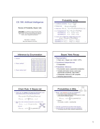
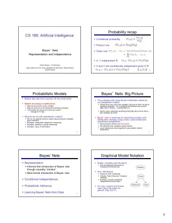
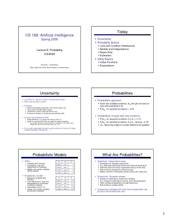
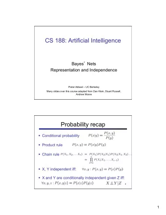
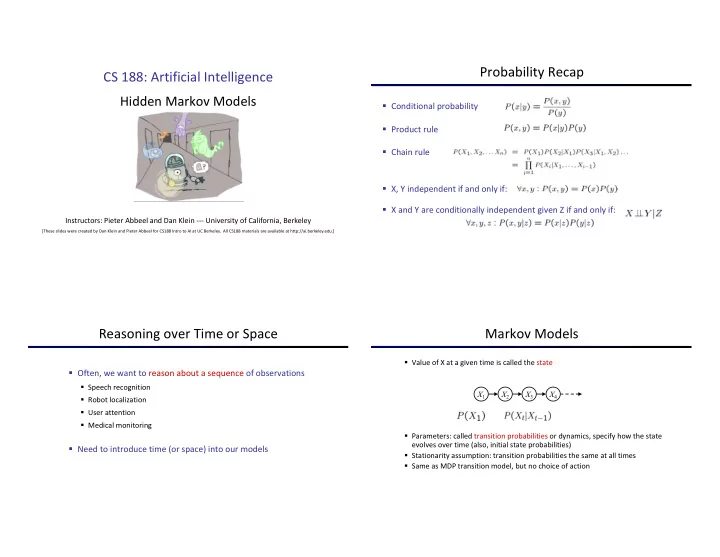
Probability Recap CS 188: Artificial Intelligence Hidden Markov Models § Conditional probability § Product rule § Chain rule § X, Y independent if and only if: § X and Y are conditionally independent given Z if and only if: Instructors: Pieter Abbeel and Dan Klein --- University of California, Berkeley [These slides were created by Dan Klein and Pieter Abbeel for CS188 Intro to AI at UC Berkeley. All CS188 materials are available at http://ai.berkeley.edu.] Reasoning over Time or Space Markov Models § Value of X at a given time is called the state § Often, we want to reason about a sequence of observations § Speech recognition X 1 X 2 X 3 X 4 § Robot localization § User attention § Medical monitoring § Parameters: called transition probabilities or dynamics, specify how the state evolves over time (also, initial state probabilities) § Need to introduce time (or space) into our models § Stationarity assumption: transition probabilities the same at all times § Same as MDP transition model, but no choice of action

Conditional Independence Example Markov Chain: Weather § States: X = {rain, sun} § Initial distribution: 1.0 sun § Basic conditional independence: § Past and future independent given the present § CPT P(X t | X t-1 ): Two new ways of representing the same CPT § Each time step only depends on the previous § This is called the (first order) Markov property X t-1 X t P(X t |X t-1 ) 0.9 0.3 0.9 sun sun 0.9 § Note that the chain is just a (growable) BN sun sun rain sun 0.1 sun rain 0.1 § We can always use generic BN reasoning on it if we 0.3 rain sun 0.3 truncate the chain at a fixed length rain rain 0.7 rain rain 0.7 0.7 0.1 Example Markov Chain: Weather Mini-Forward Algorithm 0.9 § Initial distribution: 1.0 sun 0.3 § Question: What’s P(X) on some day t? rain sun X 1 X 2 X 3 X 4 0.7 0.1 § What is the probability distribution after one step? P ( x t ) = X P ( x t − 1 , x t ) x t − 1 X = P ( x t | x t − 1 ) P ( x t − 1 ) x t − 1 Forward simulation

Video of Demo Ghostbusters Basic Dynamics Example Run of Mini-Forward Algorithm § From initial observation of sun P( X 1 ) P( X 2 ) P( X 3 ) P( X 4 ) P( X ¥ ) § From initial observation of rain P( X 1 ) P( X 2 ) P( X 3 ) P( X 4 ) P( X ¥ ) § From yet another initial distribution P(X 1 ): … P( X 1 ) P( X ¥ ) [Demo: L13D1,2,3] Video of Demo Ghostbusters Circular Dynamics Video of Demo Ghostbusters Whirlpool Dynamics

Stationary Distributions Example: Stationary Distributions § Question: What’s P(X) at time t = infinity? § For most chains: § Stationary distribution: § Influence of the initial distribution § The distribution we end up with is called X 1 X 2 X 3 X 4 gets less and less over time. the stationary distribution of the P ∞ chain § The distribution we end up in is P ∞ ( sun ) = P ( sun | sun ) P ∞ ( sun ) + P ( sun | rain ) P ∞ ( rain ) independent of the initial distribution § It satisfies P ∞ ( rain ) = P ( rain | sun ) P ∞ ( sun ) + P ( rain | rain ) P ∞ ( rain ) X P ∞ ( X ) = P ∞ +1 ( X ) = P ( X | x ) P ∞ ( x ) P ∞ ( sun ) = 0 . 9 P ∞ ( sun ) + 0 . 3 P ∞ ( rain ) X t-1 X t P(X t |X t-1 ) x P ∞ ( rain ) = 0 . 1 P ∞ ( sun ) + 0 . 7 P ∞ ( rain ) sun sun 0.9 sun rain 0.1 P ∞ ( sun ) = 3 P ∞ ( rain ) rain sun 0.3 P ∞ ( rain ) = 1 / 3 P ∞ ( sun ) P ∞ ( sun ) = 3 / 4 rain rain 0.7 Also: P ∞ ( rain ) = 1 / 4 P ∞ ( sun ) + P ∞ ( rain ) = 1 Application of Stationary Distribution: Web Link Analysis Application of Stationary Distributions: Gibbs Sampling* § PageRank over a web graph § Each joint instantiation over all hidden and query § Each web page is a state variables is a state: {X 1 , …, X n } = H U Q § Initial distribution: uniform over pages § Transitions: § Transitions: § With prob. c, uniform jump to a § With probability 1/n resample variable X j according to random page (dotted lines, not all shown) § With prob. 1-c, follow a random P(X j | x 1 , x 2 , …, x j-1, x j+1 , …, x n, e 1, … , e m ) outlink (solid lines) § Stationary distribution § Stationary distribution: § Will spend more time on highly reachable pages § Conditional distribution P(X 1 , X 2 , … , X n |e 1, … , e m ) § E.g. many ways to get to the Acrobat Reader download page § Means that when running Gibbs sampling long enough § Somewhat robust to link spam we get a sample from the desired distribution § Google 1.0 returned the set of pages containing all your keywords in decreasing rank, now all search engines use link § Requires some proof to show this is true! analysis along with many other factors (rank actually getting less important over time)

Hidden Markov Models Pacman – Sonar (P4) [Demo: Pacman – Sonar – No Beliefs(L14D1)] Video of Demo Pacman – Sonar (no beliefs) Hidden Markov Models § Markov chains not so useful for most agents § Need observations to update your beliefs § Hidden Markov models (HMMs) § Underlying Markov chain over states X § You observe outputs (effects) at each time step X 1 X 2 X 3 X 4 X 5 E 1 E 2 E 3 E 4 E 5

Example: Weather HMM Example: Ghostbusters HMM P ( X t | X t − 1 ) § P(X 1 ) = uniform 1/9 1/9 1/9 Rain t-1 Rain t Rain t+1 1/9 1/9 1/9 P(X|X � ) = usually move clockwise, but § P ( E t | X t ) 1/9 1/9 1/9 sometimes move in a random direction or stay in place Umbrella t-1 P(X 1 ) Umbrella t Umbrella t+1 § P(R ij |X) = same sensor model as before: 1/6 1/6 1/2 red means close, green means far away. 0 1/6 0 § An HMM is defined by: R t-1 R t P(R t |R t-1 ) R t U t P(U t |R t ) X 1 X 2 X 3 X 4 0 0 0 § Initial distribution: +r +r 0.7 +r +u 0.9 +r -r 0.3 +r -u 0.1 § Transitions: P(X|X � =<1,2>) P ( X t | X t − 1 ) X 5 -r +r 0.3 -r +u 0.2 § Emissions: P ( E t | X t ) R i,j R i,j R i,j R i,j -r -r 0.7 -r -u 0.8 [Demo: Ghostbusters – Circular Dynamics – HMM (L14D2)] Conditional Independence Video of Demo Ghostbusters – Circular Dynamics -- HMM § HMMs have two important independence properties: § Markov hidden process: future depends on past via the present § Current observation independent of all else given current state X 1 X 2 X 3 X 4 X 5 E 1 E 2 E 3 E 4 E 5 § Quiz: does this mean that evidence variables are guaranteed to be independent? § [No, they tend to correlated by the hidden state]

Real HMM Examples Filtering / Monitoring § Speech recognition HMMs: § Filtering, or monitoring, is the task of tracking the distribution § Observations are acoustic signals (continuous valued) B t (X) = P t (X t | e 1 , …, e t ) (the belief state) over time § States are specific positions in specific words (so, tens of thousands) § Machine translation HMMs: § We start with B 1 (X) in an initial setting, usually uniform § Observations are words (tens of thousands) § States are translation options § As time passes, or we get observations, we update B(X) § Robot tracking: § The Kalman filter was invented in the 60’s and first § Observations are range readings (continuous) § States are positions on a map (continuous) implemented as a method of trajectory estimation for the Apollo program Example: Robot Localization Example: Robot Localization Example from Michael Pfeiffer Prob 0 1 Prob 0 1 t=1 t=0 Sensor model: can read in which directions there is a wall, Lighter grey: was possible to get the reading, but less likely b/c never more than 1 mistake required 1 mistake Motion model: may not execute action with small prob.

Example: Robot Localization Example: Robot Localization Prob 0 1 Prob 0 1 t=2 t=3 Example: Robot Localization Example: Robot Localization Prob 0 1 Prob 0 1 t=4 t=5

Passage of Time Inference: Base Cases § Assume we have current belief P(X | evidence to date) X 1 X 2 X 1 X 1 X 2 § Then, after one time step passes: E 1 X P ( X t +1 | e 1: t ) = P ( X t +1 , x t | e 1: t ) x t § Or compactly: X = P ( X t +1 | x t , e 1: t ) P ( x t | e 1: t ) x t X B 0 ( X t +1 ) = P ( X 0 | x t ) B ( x t ) X = P ( X t +1 | x t ) P ( x t | e 1: t ) x t x t § Basic idea: beliefs get “pushed” through the transitions § With the “B” notation, we have to be careful about what time step t the belief is about, and what evidence it includes Example: Passage of Time Observation § Assume we have current belief P(X | previous evidence): X 1 § As time passes, uncertainty � accumulates � (Transition model: ghosts usually go clockwise) B 0 ( X t +1 ) = P ( X t +1 | e 1: t ) E 1 § Then, after evidence comes in: P ( X t +1 | e 1: t +1 ) = P ( X t +1 , e t +1 | e 1: t ) /P ( e t +1 | e 1: t ) ∝ X t +1 P ( X t +1 , e t +1 | e 1: t ) T = 1 T = 2 T = 5 = P ( e t +1 | e 1: t , X t +1 ) P ( X t +1 | e 1: t ) = P ( e t +1 | X t +1 ) P ( X t +1 | e 1: t ) § Basic idea: beliefs “reweighted” § Or, compactly: by likelihood of evidence § Unlike passage of time, we have B ( X t +1 ) ∝ X t +1 P ( e t +1 | X t +1 ) B 0 ( X t +1 ) to renormalize