Probability & Language Modeling (II) Classification & the - PowerPoint PPT Presentation
Probability & Language Modeling (II) Classification & the Noisy Channel Model CMSC 473/673 UMBC September 11 th , 2017 Some slides adapted from 3SLP , Jason Eisner Recap from last time Three people have been fatally shot, p (
n = 3 His employer , if silver was regulated according to the temporary and occasional event . What goods could bear the expense of defending themselves , than in the value of different sorts of goods , and placed at a much greater , there have been the effects of self-deception , this attention , but a very important ones , and which , having become of less than they ever were in this agreement for keeping up the business of weighing . After food , clothes , and a few months longer credit than is wanted , there must be sufficient to keep by him , are of such colonies to surmount . They facilitated the acquisition of the empire , both from the rents of land and labour of those pedantic pieces of silver which he can afford to take from the duty upon every quarter which they have a more equable distribution of employment .
n = 4 To buy in one market , in order to have it ; but the 8th of George III . The tendency of some of the great lords , gradually encouraged their villains to make upon the prices of corn , cattle , poultry , etc . Though it may , perhaps , in the mean time , that part of the governments of New England , the market , trade cannot always be transported to so great a number of seamen , not inferior to those of other European nations from any direct trade to America . The farmer makes his profit by parting with it . But the government of that country below what it is in itself necessarily slow , uncertain , liable to be interrupted by the weather .
0s Are Not Your (Language Model’s) Friend 𝑞 item ∝ 𝑑𝑝𝑣𝑜𝑢 item = 0 → 𝑞 item = 0
0s Are Not Your (Language Model’s) Friend 𝑞 item ∝ 𝑑𝑝𝑣𝑜𝑢 item = 0 → 𝑞 item = 0 0 probability item is impossible 0s annihilate: x*y*z*0 = 0 Language is creative: new words keep appearing existing words could appear in known contexts How much do you trust your data?
Add- λ estimation Laplace smoothing, Lidstone smoothing Pretend we saw each word λ more times than we did Add λ to all the counts
Add- λ estimation Laplace smoothing, Lidstone smoothing Pretend we saw each word λ more times than we did Add λ to all the counts
Add- λ estimation Laplace smoothing, Lidstone smoothing Pretend we saw each word λ more times than we did Add λ to all the counts
Add- λ estimation Laplace smoothing, Lidstone smoothing Pretend we saw each word λ more times than we did Add λ to all the counts
Add- λ N-Grams (Unigrams) The film got a great opening and the film went on to become a hit . Word (Type) Raw Count Norm Prob. Add- λ Count Add- λ Norm. Add- λ Prob. The 1 1/16 film 2 1/8 got 1 1/16 a 2 1/8 great 1 1/16 opening 1 1/16 and 1 1/16 16 the 1 1/16 went 1 1/16 on 1 1/16 to 1 1/16 become 1 1/16 hit 1 1/16 . 1 1/16
Add-1 N-Grams (Unigrams) The film got a great opening and the film went on to become a hit . Word (Type) Raw Count Norm Prob. Add-1 Count Add-1 Norm. Add-1 Prob. The 1 1/16 2 film 2 1/8 3 got 1 1/16 2 a 2 1/8 3 great 1 1/16 2 opening 1 1/16 2 and 1 1/16 2 16 the 1 1/16 2 went 1 1/16 2 on 1 1/16 2 to 1 1/16 2 become 1 1/16 2 hit 1 1/16 2 . 1 1/16 2
Add-1 N-Grams (Unigrams) The film got a great opening and the film went on to become a hit . Word (Type) Raw Count Norm Prob. Add-1 Count Add-1 Norm. Add-1 Prob. The 1 1/16 2 film 2 1/8 3 got 1 1/16 2 a 2 1/8 3 great 1 1/16 2 opening 1 1/16 2 and 1 1/16 2 16 + 14*1 = 16 30 the 1 1/16 2 went 1 1/16 2 on 1 1/16 2 to 1 1/16 2 become 1 1/16 2 hit 1 1/16 2 . 1 1/16 2
Add-1 N-Grams (Unigrams) The film got a great opening and the film went on to become a hit . Word (Type) Raw Count Norm Prob. Add-1 Count Add-1 Norm. Add-1 Prob. The 1 1/16 2 =1/15 film 2 1/8 3 =1/10 got 1 1/16 2 =1/15 a 2 1/8 3 =1/10 great 1 1/16 2 =1/15 opening 1 1/16 2 =1/15 and 1 1/16 2 =1/15 16 + 14*1 = 16 30 the 1 1/16 2 =1/15 went 1 1/16 2 =1/15 on 1 1/16 2 =1/15 to 1 1/16 2 =1/15 become 1 1/16 2 =1/15 hit 1 1/16 2 =1/15 . 1 1/16 2 =1/15
Backoff and Interpolation Sometimes it helps to use less context condition on less context for contexts you haven’ t learned much
Backoff and Interpolation Sometimes it helps to use less context condition on less context for contexts you haven’ t learned much about Backoff: use trigram if you have good evidence otherwise bigram, otherwise unigram
Backoff and Interpolation Sometimes it helps to use less context condition on less context for contexts you haven’ t learned much about Backoff: use trigram if you have good evidence otherwise bigram, otherwise unigram Interpolation: mix (average) unigram, bigram, trigram
Linear Interpolation Simple interpolation 𝑞 𝑧 𝑦) = 𝜇𝑞 2 𝑧 𝑦) + 1 − 𝜇 𝑞 1 𝑧 0 ≤ 𝜇 ≤ 1
Linear Interpolation Simple interpolation 𝑞 𝑧 𝑦) = 𝜇𝑞 2 𝑧 𝑦) + 1 − 𝜇 𝑞 1 𝑧 0 ≤ 𝜇 ≤ 1 Condition on context 𝑞 𝑨 𝑦, 𝑧) = 𝜇 3 𝑦, 𝑧 𝑞 3 𝑨 𝑦, 𝑧) + 𝜇 2 (𝑧)𝑞 2 𝑨 | 𝑧 + 𝜇 1 𝑞 1 (𝑨)
Backoff Trust your statistics, up to a point
Discounted Backoff Trust your statistics, up to a point
Discounted Backoff Trust your statistics, up to a point discount constant context-dependent normalization constant
Setting Hyperparameters Use a development corpus Dev Test Training Data Data Data Choose λs to maximize the probability of dev data: Fix the N-gram probabilities/counts (on the training data) Search for λs that give largest probability to held-out set
Implementation: Unknown words Create an unknown word token <UNK> Training: 1. Create a fixed lexicon L of size V 2. Change any word not in L to <UNK> 3. Train LM as normal Evaluation: Use UNK probabilities for any word not in training
Other Kinds of Smoothing Interpolated (modified) Kneser-Ney Idea: How “productive” is a context? How many different word types v appear in a context x, y Good-Turing Partition words into classes of occurrence Smooth class statistics Properties of classes are likely to predict properties of other classes Witten-Bell Idea: Every observed type was at some point novel Give MLE prediction for novel type occurring
Bayes Rule NLP Applications prior likelihood probability posterior probability marginal likelihood (probability)
Text Classification Assigning subject Age/gender identification categories, topics, or Language Identification genres Sentiment analysis Spam detection … Authorship identification
Text Classification Assigning subject Age/gender identification categories, topics, or Language Identification genres Sentiment analysis Spam detection … Authorship identification Input : a document a fixed set of classes C = { c 1 , c 2 ,…, c J } Output : a predicted class c C
Text Classification: Hand-coded Rules? Assigning subject Age/gender identification categories, topics, or Language Identification genres Sentiment analysis Spam detection … Authorship identification Rules based on combinations of words or other features spam: black-list- address OR (“dollars” AND“have been selected”) Accuracy can be high If rules carefully refined by expert Building and maintaining these rules is expensive
Text Classification: Supervised Machine Learning Assigning subject Age/gender identification categories, topics, or Language Identification genres Sentiment analysis Spam detection … Authorship identification Input: a document d a fixed set of classes C = { c 1 , c 2 ,…, c J } A training set of m hand-labeled documents (d 1 ,c 1 ),....,(d m ,c m ) Output: a learned classifier γ:d c
Text Classification: Supervised Machine Learning Assigning subject Age/gender identification categories, topics, or Language Identification genres Sentiment analysis Spam detection … Authorship identification Input: Naïve Bayes a document d Logistic regression a fixed set of classes C = { c 1 , c 2 ,…, c J } Support-vector A training set of m hand-labeled documents (d 1 ,c 1 ),....,(d m ,c m ) machines Output: k-Nearest Neighbors a learned classifier γ:d c …
Text Classification: Supervised Machine Learning Assigning subject Age/gender identification categories, topics, or Language Identification genres Sentiment analysis Spam detection … Authorship identification Input: Naïve Bayes a document d Logistic regression a fixed set of classes C = { c 1 , c 2 ,…, c J } Support-vector A training set of m hand-labeled documents (d 1 ,c 1 ),....,(d m ,c m ) machines Output: k-Nearest Neighbors a learned classifier γ:d c …
Probabilistic Text Classification Assigning subject Age/gender identification categories, topics, or Language Identification genres Sentiment analysis Spam detection … Authorship identification class observed data
Probabilistic Text Classification Assigning subject Age/gender identification categories, topics, or Language Identification genres Sentiment analysis Spam detection … Authorship identification prior class-based probability of likelihood class class observed observation likelihood (averaged over all classes) data
Noisy Channel Model
Noisy Channel Model what I want to tell you “sports”
Noisy Channel Model what you what I want to actually see tell you “The Os lost “sports” again…”
Noisy Channel Model Decode hypothesized what you what I want to intent actually see tell you “sad stories” “The Os lost “sports” “sports” again…”
Noisy Channel Model Decode Rerank hypothesized reweight what you what I want to intent according to actually see tell you “sad stories” what’s likely “The Os lost “sports” “sports” “sports” again…”
Noisy Channel Machine translation Part-of-speech tagging Speech-to-text Morphological analysis Spelling correction … Text normalization translation/ (clean) possible decode language (clean) model model output observed observation (noisy) likelihood (noisy) text
Noisy Channel Machine translation Part-of-speech tagging Speech-to-text Morphological analysis Spelling correction … Text normalization translation/ (clean) possible decode language (clean) model model output observed observation (noisy) likelihood (noisy) text
Language Model Use any of the language modeling algorithms we’ve learned Unigram, bigram, trigram Add- λ , interpolation, backoff (Later: Maxent , RNNs, hierarchical Bayesian LMs, …)
Noisy Channel
Noisy Channel
Noisy Channel constant with respect to X
Recommend
More recommend
Explore More Topics
Stay informed with curated content and fresh updates.
