Probability and Statistics for Computer Science Who discovered - PowerPoint PPT Presentation

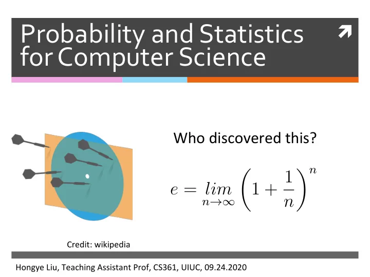
Probability and Statistics ì for Computer Science Who discovered this? � n � 1 + 1 e = lim n n →∞ Credit: wikipedia Hongye Liu, Teaching Assistant Prof, CS361, UIUC, 09.24.2020

Last time ✺ Random Variable ✺ Review with ques,ons ✺ The weak law of large numbers

Proof of Weak law of large numbers ✺ Apply Chebyshev’s inequality P ( | X − E [ X ] | ≥ � ) ≤ var [ X ] � 2 var [ X ] = var [ X ] ✺ SubsQtute and E [ X ] = E [ X ] N P ( | X − E [ X ] | ≥ � ) ≤ var [ X ] 0 N � 2 N → ∞ N →∞ P ( | X − E [ X ] | ≥ � ) = 0 lim

Applications of the Weak law of large numbers

Applications of the Weak law of large numbers ✺ The law of large numbers jus$fies using simula$ons (instead of calculaQon) to esQmate the expected values of random variables N →∞ P ( | X − E [ X ] | ≥ � ) = 0 lim ✺ The law of large numbers also jus$fies using histogram of large random samples to approximate the probability distribuQon funcQon , see proof on P ( x ) Pg. 353 of the textbook by DeGroot, et al.

Histogram of large random IID samples approximates the probability distribution ✺ The law of large numbers jusQfies using histograms to approximate the probability distribuQon. Given N IID random variables X 1 , …, X N ✺ According to the law of large numbers � N i =1 Y i N → ∞ E [ Y i ] Y = N ✺ As we know for indicator funcQon E [ Y i ] = P ( c 1 ≤ X i < c 2 ) = P ( c 1 ≤ X < c 2 )

Simulation of the sum of two-dice ✺ hZp://www.randomservices.org/ random/apps/DiceExperiment.html

Probability using the property of Independence: Airline overbooking ✺ An airline has a flight with s seats. They always sell t ( t > s ) Qckets for this flight. If Qcket holders show up independently with probability p , what is the probability that the flight is overbooked ? t � P( overbooked) C ( t, u ) p u (1 − p ) t − u = u = s +1

Simulation of airline overbooking ✺ An airline has a flight with 7 seats. They always sell 12 Qckets for this flight. If Qcket holders show up independently with probability p , esQmate the following values ✺ Expected value of the number of Qcket holders who show up ✺ Probability that the flight being overbooked ✺ Expected value of the number of Qcket holders who can’t fly due to the flight is overbooked.

Conditional expectation ✺ Expected value of X condiQoned on event A: � E [ X | A ] = xP ( X = x | A ) x ∈ D ( X ) ✺ Expected value of the number of Qcketholders not flying t � t � p u (1 − p ) t − u � u ( u − s ) E [ NF | overbooked ] = � t � t � p v (1 − p ) t − v v = s +1 u = s +1 v

Simulate the arrival ✺ Expected value of the number of Qcket holders who show up nt=100000, t= 12, s=7, p=0.1, 0.2, … 1.0 Num of trials ( nt ) … Num of Qckets (t) We generate a matrix of random numbers from uniform distribuQon in [0,1], . . Any number < p is . considered an arrival

Simulate the arrival ✺ Expected value of the number of Qcket holders who show up Expected value of the number of ticket holders who show up 12 nt=100000, t= 12, ● ● s=7, p=0.1, 0.2, … 1.0 10 ● ● 8 Expected value ● 6 ● ● 4 ● ● 2 ● 0.2 0.4 0.6 0.8 1.0 Probability of arrival (p)

Simulate the expected probability of overbooking ✺ Expected probability of the flight being overbooked t= 12, s=7, p=0.1, 0.2, … 1.0 ✺ Expected probability is equal to the expected value of indicator func:on . Whenever we have Num of arrival > Num of seats, we mark it with an indicator funcQon. Then esQmate with the sample mean of indicator funcQons.

Simulate the expected probability of overbooking ✺ Expected probability of the Expected probability of flight being overbooked 1.0 ● ● flight being ● overbooked 0.8 ● 0.6 Expected value nt=100000, ● 0.4 t= 12, s=7, p=0.1, 0.2, … 1.0 0.2 ● ● 0.0 ● ● ● 0.2 0.4 0.6 0.8 1.0 Probability of arrival (p)

Simulate the expected value of the number of grounded ticket holders given overbooked ✺ Expected value of the number of Qcket Expected value of the number of ticket holder not flying given overbooked ● 5 holders who can’t fly due to the flight 4 ● being overbooked Expected value 3 ● Nt=200000, ● t= 12, s=7, 2 ● p=0.1, 0.2, … 1.0 ● ● ● ● 1 ● 0.2 0.4 0.6 0.8 1.0 Probability of arrival (p)

Content ✺ Con:nuous Random Variable ✺ Important known discrete probability distribuQons

Example of a continuous random variable ✺ The spinner θ θ ∈ (0 , 2 π ] 0 ✺ The sample space for all outcomes is not countable

Probability density function (pdf) ✺ For a conQnuous random variable X, the probability that X = x is essenQally zero for all (or most) x , so we can’t define P ( X = x ) ✺ Instead, we define the probability density func:on (pdf) over an infinitesimally small interval dx, p ( x ) dx = P ( X ∈ [ x, x + dx ]) � b ✺ For a < b p ( x ) dx = P ( X ∈ [ a, b ]) a

Properties of the probability density function ✺ resembles the probability funcQon p ( x ) of discrete random variables in that ✺ for all x p ( x ) ≥ 0 ✺ The probability of X taking all possible values is 1. � ∞ p ( x ) dx = 1 −∞

Properties of the probability density function ✺ differs from the probability p ( x ) distribuQon funcQon for a discrete random variable in that ✺ is not the probability that X = x p ( x ) ✺ can exceed 1 p ( x )

Probability density function: spinner ✺ Suppose the spinner has equal chance stopping at any posiQon. What’s the pdf of the angle θ of the spin posiQon? c � if θ ∈ (0 , 2 π ] c p ( θ ) = 0 otherwise 0 2π θ ✺ For this funcQon to be a pdf, Then � ∞ p ( θ ) d θ = 1 −∞

Probability density function: spinner ✺ What the probability that the spin angle θ is within [ ]? 12 , π π 7

Q: Probability density function: spinner ✺ What is the constant c given the spin angle θ has the following pdf? p ( θ ) A. 1 B. 1/π C. 2/π c D. 4/π E. 1/2π π 0 2π θ

Expectation of continuous variables ✺ Expected value of a conQnuous random variable X weight � ∞ E [ X ] = xp ( x ) dx x −∞ ✺ Expected value of funcQon of conQnuous random variable Y = f ( X ) � ∞ E [ Y ] = E [ f ( X )] = f ( x ) p ( x ) dx −∞

Probability density function: spinner ✺ Given the probability density of the spin angle θ � 1 if θ ∈ (0 , 2 π ] p ( θ ) = 2 π 0 otherwise ✺ The expected value of spin angle is � ∞ E [ θ ] = θ p ( θ ) d θ −∞

Properties of expectation of continuous random variables ✺ The linearity of expected value is true for conQnuous random variables. � � ✺ And the other properQes that we derived for variance and covariance also hold for conQnuous random variable

Q. ✺ Suppose a conQnuous variable has pdf � 2(1 − x ) x ∈ [0 , 1] p ( x ) = 0 otherwise What is E[X]? A. 1/2 B. 1/3 C. 1/4 D. 1 E. 2/3 � ∞ E [ X ] = xp ( x ) dx −∞

Variance of a continuous variable

Content ✺ ConQnuous Random Variable ✺ Important known discrete probability distribu:ons

The usefulness of probability distributions ✺ Many common processes generate data with probability distribuQons that belong to families with known properQes ✺ Even if the data are not distributed according to a known probability distribuQon, it is someQmes useful in pracQce to approximate with known distribuQon.

The classic discrete distributions

Discrete uniform distribution ✺ A discrete random variable X is uniform if it takes k different values and P ( X = x i ) = 1 For all x i that X can take k ✺ For example: ✺ Rolling a fair k-sided die ✺ Tossing a fair coin (k=2)

Discrete uniform distribution ✺ ExpectaQon of a discrete random variable X that takes k different values uniformly k E [ X ] = 1 � x i k i =1 ✺ Variance of a uniformly distributed random variable X . k var [ X ] = 1 � ( x i − E [ X ]) 2 k i =1

Bernoulli distribution ✺ A random variable X is Bernoulli if it takes on two values 0 and 1 such that E [ X ] = p var [ X ] = p (1 − p ) Jacob Bernoulli (1654-1705) Credit: wikipedia

Bernoulli distribution ✺ Examples ✺ Tossing a biased (or fair) coin ✺ Making a free throw ✺ Rolling a six-sided die and checking if it shows 6 ✺ Any indicator func:on of a random variable

Binomial distribution ✺ Remember Galton Board? hZp://www.randomservices.org/ random/apps/ GaltonBoardExperiment.html ✺ Remember the airline problem?

Binomial distribution P = 0.5 Credit: Prof. Grinstead

Binomial distribution ✺ A discrete random variable X is binomial if � N � p k (1 − p ) N − k P ( X = k ) = for integer 0 ≤ k ≤ N k with E [ X ] = Np & var [ X ] = Np (1 − p ) ✺ Examples ✺ If we roll a six-sided die N Qmes, how many sixes we will see ✺ If I aZempt N free throws, how many points will I score ✺ What is the sum of N independent and iden:cally distributed Bernoulli trials?

Expectations of Binomial distribution ✺ A discrete random variable X is binomial if � N � p k (1 − p ) N − k P ( X = k ) = for integer 0 ≤ k ≤ N k with E [ X ] = Np & var [ X ] = Np (1 − p )