Probability and Statistics for Computer Science The weak law of - PowerPoint PPT Presentation

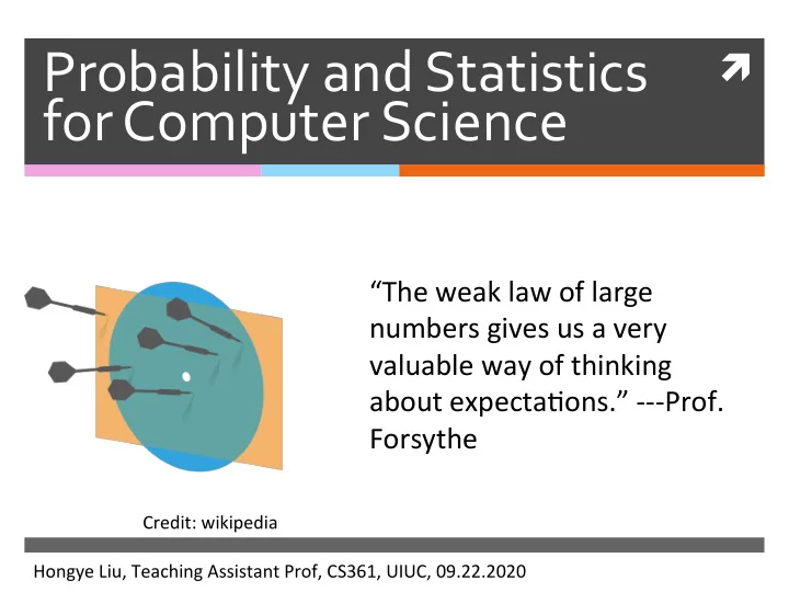
Probability and Statistics ì for Computer Science “The weak law of large numbers gives us a very valuable way of thinking about expecta:ons.” ---Prof. Forsythe Credit: wikipedia Hongye Liu, Teaching Assistant Prof, CS361, UIUC, 09.22.2020

Midtemexau.li# on0c € schedule Please CBTFexamzpract.is are 2 Solutions problem linked a

will be given practice exam One Grades cope co through week in a protocol CBTF exam mimic .

How many colors possible ? Hexadecimal Kolar codes Hex uses define colors per position ) ( 16 to format . colors how 9 - digits , many Here With . be represented ? can ( 69,4 × 9 eb 16 × 16 x . - .

Last time c R - V . ) variable Random Xcw ) * Definition value Expected properties f CX ) * - fix . 's ) & covariance Variance * #

Objectives , R Random variable expectations of * Review Markov 's Inequality * 's inequality chebyshev Lyga numbers law of weak * The

Expected value � The expected value (or expecta,on ) of a random variable X is Pc ¥ " � E [ X ] = xP ( x ) x The expected value is a weighted sum of all the values X can take

Linearity of Expectation E- ( a Xtb ] = a Etat b EAT t EET ) Ef Xt Y ] = = ? Efxi ] E [ ? Xi )

Expected value of a function of X . Pix ) Eff CX ) ) = I fix ) 7C

Probability distribution � Given the random variable X , what is E- ( 21 × 41 ] =2Eh × =3 E[2| X | +1]? El 1 × 11=7 " t - EY , * ÷ - z Hmp ' " A. 0 p ( x ) P ( X = x ) B. 1 =/ C. 2 D. 3 a 1/2 E. 5 0 -1 1 X

Expected time of cat � A cat moves with random constant speed V , either 5mile/hr or 20mile/hr with equal probability, what’s the expected 5me for it to travel 50 miles? D- = f ' V ) T = Earl a • vs t EITI Z type . Paris + ¥ . p cuz , = ÷ xtz-6.rs x 'T t =

inequality Jensen 's g. CX ) tune convex . for Elgin ) > glean ) # assume Can 't ELgcxst-glEHD.iq -

A neater expression for variance � Variance of Random Variable X is defined as: var [ X ] = E [( X − E [ X ]) 2 ] vague XI = ? thevar Ex ] � It’s the same as: A var [ X ] = E [ X 2 ] − E [ X ] 2

Probability distribution and cumulative distribution � Given the random variable X , what is = Ivar ( I xp ] var[2| X | +1]? I A. 0 p ( x ) P ( X = x ) B. 1 C. 2 D. 3 1/2 E. -1 0 -1 1 X •

Probability distribution � Given the random variable X , what is var[2| X | +1]? Let Y = 2| X |+1 . I txt ) i p ( y ) P ( Y = y ) - EH xD ' ] Eflxl = - 1 0 3 X

Probability distribution � Given the random variable X , what is var[2| X | +1]? Let Y = 2| X |+1 p ( y ) P ( Y = y ) 1 0 3 X

Probability distribution � Give the random variable S in the 4- sided die, whose range is {2,3,4,5,6,7,8}, probability distribu:on of S. - p ( s ) What is var[S] ? ECS 't - Ecs ) =ZEgED 1/16 S 5 6 8 2 3 4 7 -

are equivalent These , -0=0 Corr CX , 41=0 ; Cov CX (1) = ECXIECY ] ECXYI ( I ) - uarfxfiuascy ] var [ Xt 's ] - ( II ) X , Y are all mean they uncorrelated . ECXTI - E- CHEH ] Cove x. ' D= var Ext 'll = usixltuarteltrcoucx , y ,

Properties of independence in terms of expectations ' fore inept . � X. E [ XY ] = E [ X ] E [ Y ] it - y ) xypcx 2- -2 LHS = Proof : x y ifX.Tareiwdpt.pl x. g) =p ex ) pay , . y ace * for = I xpcac , Egg pigs LH s = RHS ECXIEIT ] =

X , T independent If are - Corr CX , -9=0 Cove X. 41=0 , then { uarfxtyj-uarcxltuas.IT ] = EAT ECT ] ECXY ) ¥±÷i÷÷÷ :

on it off line work Q: What is this expectation? � We toss two iden5cal coins A & B independently for three 5mes and 4 5mes respec5vely, for each head we earn $1, we define X is the earning from A and Y is the earning from B. What is E( XY )? K D ECx7= ? ECT ) = ? A. $2 B. $3 C. $4

it offline Work on Uncorrelated vs Independent � If two random variables are uncorrelated, does this mean they are independent? Inves5gate the case X takes -1, 0, 1 with equal probability and Y=X 2 . -_ Efx ) ECT ) E- Cx 's pck.gl#Pcxspcy ) but

do you with die ? make How it a as it biased wig throwing a head ? coming -_ 0.75 probability up with 4 - sided die 0.25 1,213 € - l T 4 - logo p -

RVs 2 mean that What does it distr . ? the scene have / " Pl X - - 24 , ,PlY=y ) Hit . identical t ÷ - . 4- die-off Yew > =/ ? tail X ( w )={ ° , head 4- die comes , odd 4- die xp 2- Cw ) =/ ° I orz shows - z I or 4 - -

Three experiments of Students 2 number each sum of the Report random 4- a fa die rolling finds after . add them roll then once each ① , + " U 't 'm Etten sit them " " s at u . times its then rolls @ once , one gamer variance 2 .

Ist M l und - 14 I . N car - die Sunny . distinct numbers - N M N = i - I t i - MX N = M N X - I ④ Nr-N X - p - µµ _C -

Towards the weak law of large numbers � The weak law says that if we repeat a random experiment many :mes, the average of the observa:ons will “converge” to the expected value � For example, if you repeat the profit example, the average earning will “converge” to E[ X ]=20p-10 - # 5 - fo � The weak law jus:fies using simula:ons (instead of calcula:on) to es:mate the expected values of E → I x. pox , random variables

Markov’s inequality � For any random variable X that only take s o - x ≥ 0 and constant a > 0 P ( X ≥ a ) ≤ E [ X ] a � For example, if a = 10 E[X] E [ X ] o P ( X ≥ 10 E [ X ]) ≤ 10 E [ X ] = 0 . 1 -

Proof of Markov’s inequality X only take a > o Expose , I Eun = X > a set a × so . " ' 3 E. age 3 I . P " ) > TP a ,a = = a. pix > a , Pity pT × ⇒ a

Chebyshev’s inequality � For any random variable X and constant a >0 P ( | X − E [ X ] | ≥ a ) ≤ var [ X ] a 2 � If we let a = kσ where σ = std[ X ] P ( | X − E [ X ] | ≥ k σ ) ≤ 1 k 2 � In words, the probability that X is greater than k standard devia:on away from the mean is small

Proof of Chebyshev’s inequality � Given Markov inequality, a>0, x ≥ 0 P ( X ≥ a ) ≤ E [ X ] a the it's same as � We can rewrite it as : ' f- IVI P ( | U | ≥ w ) ≤ E [ | U | ] ω > 0 O y 7 w U = ( X - ECHR ( x - Efx ) 5 ( VI =

Proof of Chebyshev’s inequality � If U = ( X − E [ X ]) 2 - BBpBEE" P ( | U | ≥ w ) ≤ E [ | U | ] = E [ U ] w w RHs=# pixewxwgsuarwxiii : ' pclx-EHIZajsva.az# w=a

Now we are closer to the law of large numbers

Sample mean and IID samples � We define the sample mean to be the X average of N random variables X 1 , …, X N . -#EEi÷i÷ � If X 1 , …, X N are independent and have iden,cal probability func:on P ( x ) . then the numbers randomly generated from them are called IID samples - � The sample mean is a random variable

Sample mean and IID samples � Assume we have a set of IID samples from N random variables X 1 , …, X N that have probability func:on P ( x ) � We use to denote the sample mean of X these IID samples ¥ ' D. � N i =1 X i , X = N

Expected value of sample mean of IID random variables E- CTX . - I � By linearity of expected value = -2 Efxi ] i N � N ] = 1 i =1 X i � E [ X ] = E [ E [ X i ] N N i =1 Eagle CX :D Ely ,7 ⇐ p* ' . II . EAT E- ( 51=4 - EAT = Efx ) - N - -

Expected value of sample mean of IID random variables � By linearity of expected value N � N ] = 1 i =1 X i � E [ X ] = E [ E [ X i ] N N i =1 ECXt-ECX.IE?IelxnI � Given each X i has iden:cal P ( x ) N E [ X ] = 1 � E [ X ] = E [ X ] N i =1

Variance of sample mean of IID random variables � By the scaling property of variance N N var [ X ] = var [ 1 X i ] = 1 � � N 2 var [ X i ] N i =1 i =1 , Xj ) ) { Hi mutual t . + varley var C Xitxu ) = var pix , , xi X. I - =urrfx µ ] , I = var Kil work - - = var EX ] varix ) = * t]=¥ . N - var Cx ]

Variance of sample mean of IID random variables � By the scaling property of variance N N var [ X ] = var [ 1 X i ] = 1 � � N 2 var [ X i ] N i =1 i =1 � And by independence of these IID random variables N var [ X ] = 1 � var [ X i ] N 2 i =1 var Cx ) = ¥ - varix ] var CI I = ¥ . N . an Cx ) =

Expected value and variance of sample mean of IID random variables � The expected value of sample mean is the same as the expected value of the distribu:on E [ X ] = E [ X ] � The variance of sample mean is the distribu:on’s variance divided by the sample size N var [ X ] = var [ X ] N

Weak law of large numbers � Given a random variable X with finite variance, probability distribu:on func:on and the P ( x ) sample mean of size N . X � For any posi:ve number � > 0 N →∞ P ( | X − E [ X ] | ≥ � ) = 0 lim � That is: the value of the mean of IID samples is very close with high probability to the expected value of the popula:on when sample size is very large

Proof of Weak law of large numbers � Apply Chebyshev’s inequality P ( | X − E [ X ] | ≥ � ) ≤ var [ X ] � 2 E- LET = Efx ) var ( II = # varix ]