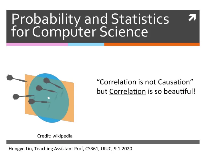
Probability and Statistics for Computer Science Correla)on is not - PowerPoint PPT Presentation

Probability and Statistics ì for Computer Science “Correla)on is not Causa)on” but Correla)on is so beau)ful! Credit: wikipedia Hongye Liu, Teaching Assistant Prof, CS361, UIUC, 9.1.2020

Last time ✺ Mean ✺ Standard devia)on ✺ Variance ✺ Standardizing data

Objectives ✺ Median, Interquar)le range, box plot and outlier ✺ ScaRer plots, Correla)on Coefficient ✺ Visualizing & Summarizing rela%onships Heatmap, 3D bar, Time series plots,

Median ✺ To organize the data we first sort it ✺ Then if the number of items N is odd median = middle item's value if the number of items N is even median = mean of middle 2 items' values

Properties of Median ✺ Scaling data scales the median median ( { k · x i } ) = k · median ( { x i } ) ✺ Transla)ng data translates the median median ( { x i + c } ) = median ( { x i } ) + c

Percentile ✺ k th percen)le is the value rela)ve to which k% of the data items have smaller or equal numbers ✺ Median is roughly the 50 th percen)le

Interquartile range ✺ iqr = (75th percen)le) - (25th percen)le) ✺ Scaling data scales the interquar)le range iqr ( { k · x i } ) = | k | · iqr ( { x i } ) ✺ Transla)ng data does NOT change the interquar)le range iqr ( { x i + c } ) = iqr ( { x i } )

Box plots Vehicle death by region ✺ Boxplots ✺ Simpler than histogram DEATH ✺ Good for outliers ✺ Easier to use for comparison Data from hRps://www2.stetson.edu/ ~jrasp/data.htm

Boxplots details, outliers ✺ How to Outlier define > 1.5 iqr Whisker outliers? (the default) Box Interquar)le Range (iqr) Median < 1.5 iqr

Sensitivity of summary statistics to outliers ✺ mean and standard devia)on are very sensi)ve to outliers ✺ median and interquar)le range are not sensi)ve to outliers

Modes ✺ Modes are peaks in a histogram ✺ If there are more than 1 mode, we should be curious as to why

Multiple modes ✺ We have seen the “iris” data which looks to have several peaks Data: “iris” in R

Example Bi-modes distribution ✺ Modes may indicate mul)ple popula)ons Data: Erythrocyte cells in healthy humans Piagnerelli, JCP 2007

Tails and Skews Credit: Prof.Forsyth

Q. How is this skewed? A Lep B Right Median = 47

Looking at relationships in data ✺ Finding rela)onships between features in a data set or many data sets is one of the most important tasks in data analysis

Relationship between data features ✺ Example: does the weight of people relate to their height? ✺ x : HIGHT, y: WEIGHT

Scatter plot ✺ Body Fat data set

Scatter plot ✺ ScaRer plot with density

Scatter plot ✺ Removed of outliers & standardized

Correlation seen from scatter plots Zero Posi)ve Nega)ve Correla)on correla)on correla)on Credit: Prof.Forsyth

What kind of Correlation? ✺ Line of code in a database and number of bugs ✺ Frequency of hand washing and number of germs on your hands ✺ GPA and hours spent playing video games ✺ earnings and happiness Credit: Prof. David Varodayan

Correlation doesn’t mean causation ✺ Shoe size is correlated to reading skills, but it doesn’t mean making feet grow will make one person read faster.

Correlation Coefficient ✺ Given a data set consis)ng of { ( x i , y i ) } items ( x 1 , y 1 ) ... ( x N , y N ) , ✺ Standardize the coordinates of each feature: x i = x i − mean ( { x i } ) y i = y i − mean ( { y i } ) � � std ( { x i } ) std ( { y i } ) ✺ Define the correla)on coefficient as: N � corr ( { ( x i , y i ) } ) = 1 x i � � y i N i =1

Correlation Coefficient x i = x i − mean ( { x i } ) y i = y i − mean ( { y i } ) � � std ( { x i } ) std ( { y i } ) � N corr ( { ( x i , y i ) } ) = 1 x i � � y i N i =1 = mean ( { � y i } ) x i �

Q: Correlation Coefficient ✺ Which of the following describe(s) correla)on coefficient correctly? A. It’s unitless B. It’s defined in standard coordinates C. Both A & B N � corr ( { ( x i , y i ) } ) = 1 x i � � y i N i =1

A visualization of correlation coefficient hRps://rpsychologist.com/d3/correla)on/ In a data set consis)ng of items { ( x i , y i ) } ( x 1 , y 1 ) ... ( x N , y N ) , shows posi)ve correla)on corr ( { ( x i , y i ) } ) > 0 shows nega)ve correla)on corr ( { ( x i , y i ) } ) < 0 shows no correla)on corr ( { ( x i , y i ) } ) = 0

Correlation seen from scatter plots Zero Posi)ve Nega)ve Correla)on correla)on correla)on Credit: Prof.Forsyth

The Properties of Correlation Coefficient ✺ The correla)on coefficient is symmetric corr ( { ( x i , y i ) } ) = corr ( { ( y i , x i ) } ) ✺ Transla)ng the data does NOT change the correla)on coefficient

The Properties of Correlation Coefficient ✺ Scaling the data may change the sign of the correla)on coefficient corr ( { ( a x i + b, c y i + d ) } ) = sign ( a c ) corr ( { ( x i , y i ) } )

The Properties of Correlation Coefficient ✺ The correla)on coefficient is bounded within [-1, 1] if and only if x i = � � corr ( { ( x i , y i ) } ) = 1 y i if and only if corr ( { ( x i , y i ) } ) = − 1 x i = − � � y i

Concept of Correlation Coefficient’s bound ✺ The correla)on coefficient can be wriRen as � N corr ( { ( x i , y i ) } ) = 1 x i � � y i N i =1 � N � � x i y i corr ( { ( x i , y i ) } ) = √ √ N N i =1 ✺ It’s the inner product of two vectors � � � � and � y 1 � y N � � x 1 x N √ √ √ √ N , ... N , ... N N

Inner product ✺ Inner product’s geometric meaning: ν 1 | ν 1 | | ν 2 | cos ( θ ) θ ν 2 ✺ Lengths of both vectors ν 1 = � � ν 2 = � � � � y 1 y N x N � x 1 � √ √ √ √ N , ... N , ... N N are 1

Bound of correlation coefficient | corr ( { ( x i , y i ) } ) | = | cos ( θ ) | ≤ 1 ν 1 θ ν 2 ν 1 = � � � � ν 2 = y 1 � y N � x N � x 1 � √ √ √ √ N , ... N , ... N N

The Properties of Correlation Coefficient ✺ Symmetric ✺ Transla)ng invariant ✺ Scaling only may change sign ✺ bounded within [-1, 1]

Using correlation to predict ✺ Cau'on ! Correla)on is NOT Causa)on Credit: Tyler Vigen

How do we go about the prediction? ✺ Removed of outliers & standardized

Using correlation to predict ✺ Given a correlated data set { ( x i , y i ) } we can predict a value that goes with p y 0 a value x 0 ✺ In standard coordinates { ( � x i , � y i ) } we can predict a value that goes with � p y 0 a value � x 0

Q: ✺ Which coordinates will you use for the predictor using correla)on? A. Standard coordinates B. Original coordinates C. Either

Linear predictor and its error ✺ We will assume that our predictor is linear y p = a � � x + b ✺ We denote the predic)on at each in the data � x i set as p � y i p = a � � y i x i + b ✺ The error in the predic)on is denoted u i p = � u i = � y i − � y i − a � y i x i − b

Require the mean of error to be zero We would try to make the mean of error equal to zero so that it is also centered around 0 as the standardized data:

Require the variance of error is minimal

Require the variance of error is minimal

Here is the linear predictor! y p = r � � x Correla)on coefficient

Prediction Formula ✺ In standard coordinates p = r � � r = corr ( { ( x i , y i ) } ) where y 0 x 0 ✺ In original coordinates y p 0 − mean ( { y i } ) = rx 0 − mean ( { x i } ) std ( { y i } ) std ( { x i } )

Root-mean-square (RMS) prediction error ✺ var ( { u i } ) = 1 − 2 ar + a 2 Given & a = r var ( { u i } ) = 1 − r 2 � ✺ mean ( { u 2 RMS error = i } ) � = var ( { u i } ) √ 1 − r 2 =

See the error through simulation hRps://rpsychologist.com/d3/correla)on/

Example: Body Fat data r = 0.513

Example: remove 2 more outliers r = 0.556

Heatmap ✺ Display matrix of data via gradient of color(s) Summariza)on of 4 loca)ons’ annual mean temperature by month

3D bar chart ✺ Transparent 3D bar chart is good for small # of samples across categories

Relationship between data feature and time ✺ Example: How does Amazon’s stock change over 1 years? take out the pair of features x: Day y: AMZN

Time Series Plot: Stock of Amazon

Scatter plot ✺ Coupled with heatmap to show a 3 rd feature

Assignments ✺ Finish reading Chapter 2 of the textbook ✺ Next )me: Probability a first look

Additional References ✺ Charles M. Grinstead and J. Laurie Snell "Introduc)on to Probability” ✺ Morris H. Degroot and Mark J. Schervish "Probability and Sta)s)cs”

See you next time See You!