Probability and Computation K. Sutner Carnegie Mellon University - PowerPoint PPT Presentation

Probability and Computation K. Sutner Carnegie Mellon University

Order Statistics 1 Circuit Evaluation � Yao’s Minimax Principle � More Randomized Algorithms * �

Rank and Order 3 Let U be some ordered universe such as the integers, rationals, strings, and so forth. It is easy to see that for any set A ⊆ U of size n there is a unique order isomorphism [ n ] ← → A → : ord ( k, A ) ← : rk ( a, A ) Note that ord ( k, A ) is trivial to compute if A is sorted. Computation of rk ( a, A ) requires to determine the cardinality of A ≤ a = { z ∈ A | z ≤ a } (which is easy if A is a sorted array and we have a pointer to a ). Sometimes it is more convenient to use ranks 0 ≤ r < n .

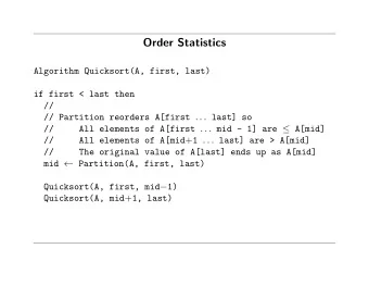
Randomized Quicksort 4 Recall randomized quicksort. For simplicity assume elements in A are unique. Pick a pivot s ∈ A uniformly at random. Partition into A <s , s , A >s . Recursively sort A <s and A >s . Here A is assumed to be given as an array. Partitioning takes linear time (though is not so easy to implement in the presence of duplicates).

Running Time 5 Let X be the random variable: size of A <s . Then p i = Pr [ X = i ] = 1 /n where i = 0 , . . . , n − 1 , n = | A | . Ignoring multiplicative constants we get � 1 if n ≤ 1 , t ( n ) = � i<n p i ( t ( i ) + t ( n − i − 1)) + n otherwise.

Simplifying 6 � � � t ( n ) = 1 /n t ( i ) + t ( n − i − 1) + n i<n � = 2 /n t ( i ) + n i<n � t ( i ) + n 2 n · t ( n ) = 2 i<n � t ( i ) + ( n + 1) 2 ( n + 1) · t ( n + 1) = 2 i ≤ n t ( n + 1) = ( n + 2) / ( n + 1) · t ( n ) + (2 n + 1) / ( n + 1) which comes down to t ( n ) = n + 1 · t ( n − 1) + 2 . n

Solving 7 t ( n ) = n + 1 /n · t ( n − 1) + 2 can be handled in to ways: Unfold the equation a few levels and observe the pattern. Solve the homogeneous equation h ( n ) = n + 1 /n · h ( n − 1) : h ( n ) = n + 1 . Then construct t from h – see any basic text on recurrence equations. Either way, we find n +1 � t ( n ) = ( n + 1) / 2 + 2( n + 1) 1 /i = Θ( n log n ) i =3

Random versus Deterministic Pivots 8 Random pivot: Pr [ X = k ] = 1 /n k = 0 , . . . , n − 1 E [ X ] = ( n − 1) / 2 Var [ X ] = ( n 2 − 1) / 12 Median of three: 6 k ( n − k − 1) Pr [ X = k ] = k = 1 , . . . , n − 2 n ( n − 1)( n − 2) E [ X ] = ( n − 1) / 2 Var [ X ] = (( n − 1) 2 − 4) / 20

Selection versus Sorting 9 While selection seems somewhat easier than sorting, it is not clear that one can avoid something like O ( n log n ) in the process of computing ord ( k, A ) . The following result was surprising. Theorem (Blum, Floyd, Pratt, Rivest, Tarjan, 1973) Selection can be handled in linear time. The algorithm is a perfectly deterministic divide-and-conquer approach. Alas, the constants are bad. Alternatively, we can use a randomized algorithm to find the k th element quickly, on average.

Probabilistic Selection 10 Given a collection A of cardinality n , a rank 0 ≤ k < n . Here is a recursive selection algorithm: Permute A in random order, yielding a 0 , a 1 , . . . , a n − 1 ; set B = nil. Pick a pivot s ∈ A at random and compute A <s and A >s . Let m = | A <s | . If k = m return s . If k < m return ord ( k, A <s ) . If k > m return ord ( k − m − 1 , A >s ) .

Running Time 11 Correctness is obvious, for the running time analysis divide [ n ] into bins of exponentially decreasing size: bin k has the form B k = [ n · (3 / 4) k , n · (3 / 4) k +1 ] where we ignore the necessary ceilings and floors, as well as overlap. Note that with probability 1 / 2 the cardinality of the selection set will move (at least) to the next bin in each round. But then it takes 2 steps on average to get (at least) to the next bin. Hence the expected number of rounds is logarithmic and the total running time therefore linear.

Order Statistics � Circuit Evaluation 2 Yao’s Minimax Principle � More Randomized Algorithms * �

Minimax Trees 13 Here is a highly simplified model of a game tree: we only consider Boolean values 2 = { 0 , 1 } and represent the two players by alternating levels of “and” and “or” gates (corresponding to min and max). More precisely, define Boolean functions T k : 2 4 k → 2 by T 1 ( x 1 , x 2 , x 3 , x 4 ) = ( x 1 ∨ x 2 ) ∧ ( x 3 ∨ x 4 ) T k +1 ( x 1 , x 2 , x 3 , x 4 ) = T 1 ( T k ( x 1 ) , T k ( x 2 ) , T k ( x 3 ) , T k ( x 4 ))

T 2 14

Lazy Evaluation 15 The Challenge: Given a truth assignment α : x → 2 , we want to evaluate the circuit T k reading as few of the bits of α as possible (think of α as a bitvector of length 4 k ). We may safely assume that we always read the input bits from left to right. For example, x 1 = x 2 = 0 already forces output 0 and we do not need to read x 3 or x 4 when evaluating T 1 . Skipping a single bit in T 1 may sound irrelevant, but skipping a whole subtree in T 3 is significant ( 16 variables). Critical parameters: R = output value S = # variables read

Augmented Truth Table 16 x 1 x 2 x 3 x 4 R S 0 0 0 0 0 2 0 0 0 1 0 2 0 0 1 0 0 2 0 0 1 1 0 2 0 1 0 0 0 4 0 1 0 1 1 4 0 1 1 0 1 3 0 1 1 1 1 3 1 0 0 0 0 3 1 0 0 1 1 3 1 0 1 0 1 2 1 0 1 1 1 2 1 1 0 0 0 3 1 1 0 1 1 3 1 1 1 0 1 2 1 1 1 1 1 2

Essential Part 17 x 1 x 2 x 3 x 4 R S 0 0 . . 0 2 0 0 . . 0 2 0 0 . . 0 2 0 0 . . 0 2 0 1 0 0 0 4 0 1 0 1 1 4 0 1 1 . 1 3 0 1 1 . 1 3 1 . 0 0 0 3 1 . 0 1 1 3 1 . 1 . 1 2 1 . 1 . 1 2 1 . 0 0 0 3 1 . 0 1 1 3 1 . 1 . 1 2 1 . 1 . 1 2

And Probability? 18 Think of choosing a truth assignment for x 1 , x 2 , x 3 , x 4 at random. R and S are now discrete random variables. Here is the PMF in the uniform case: R \ S 1 2 3 4 0 0 1 / 4 1 / 8 1 / 16 1 0 1 / 4 1 / 4 1 / 16 E [ R ] = 9 / 16 ≈ 0 . 56 E [ S ] = 21 / 8 ≈ 2 . 63

A Bound 19 Lemma E [ S k ] = 3 k = n log 4 3 ≈ n 0 . 79 Proof. Homework. ✷

Biased Input 20 How about input with bias Pr [ x = 1] = p for some 0 ≤ p ≤ 1 ? This is the bias for the original inputs at the input level of the circuit. Note that this question is really inevitable: we have to worry about the influence of T 1 gates, even if the original bias is just 1/2.

Table for Biased Input 21 x 1 x 2 x 3 x 4 R S Pr q 4 0 0 0 0 0 2 pq 3 0 0 0 1 0 2 pq 3 0 0 1 0 0 2 p 2 q 2 0 0 1 1 0 2 pq 3 0 1 0 0 0 4 p 2 q 2 0 1 0 1 1 4 p 2 q 2 0 1 1 0 1 3 p 3 q 0 1 1 1 1 3 pq 3 1 0 0 0 0 3 p 2 q 2 1 0 0 1 1 3 p 2 q 2 1 0 1 0 1 2 p 3 q 1 0 1 1 1 2 p 2 q 2 1 1 0 0 0 3 p 3 q 1 1 0 1 1 3 p 3 q 1 1 1 0 1 2 p 4 1 1 1 1 1 2

Biased Input 22 It follows that for input with bias Pr [ x = 1] = p we have E [ R 1 ] = Pr [ R 1 = 1] = p 2 (4 − 4 p + p 2 ) Sanity check: p 2 (4 − 4 p + p 2 ) [ p �→ 1 / 2] = 9 / 16 . Claim √ T 1 increases the bias for p ≥ (3 − 5) / 2 ≈ 0 . 38 . This is vaguely plausible since both “and” and “or” are monotonic. See the next plot.

p 2 (4 − 4 p + p 2 ) 23 1.0 0.8 0.6 0.4 0.2 0.2 0.4 0.6 0.8 1.0

Order Statistics � Circuit Evaluation � Yao’s Minimax Principle 3 More Randomized Algorithms * �

So What? 25 So the canonical lazy algorithm has E [ S k ] = 3 k ≈ n 0 . 79 . This may sound good, but it would be nice to have a lower bound that indicates how good this result actually is. It would be even nicer to have some general method for doing this.

Yao’s Minimax Principle 26 One can use understanding of the performance of deterministic algorithms to obtain lower bounds on the performance of probabilistic algorithms. To make this work, focus on Las Vegas algorithms: the answer is always correct, but the running time may be bad, with small probability. Given some input I , a Las Vegas algorithm A makes a sequence of random choices during execution. We can think of these choices as represented by a choice sequence C ∈ 2 ⋆ . Given I and C , the algorithm behaves in an entirely deterministic fashion: A ( I ; C ) .

Inputs and Algorithms 27 Fix some input size n once and for all (unless you love useless subscripts). I = collection of all inputs of size n A = collection of all deterministic algorithms for I It is clear that I is finite, but it requires a fairly delicate definition of “algorithm” to make sure that A is also finite. Exercise Figure out how to make sure A is finite.

LV as a Distribution 28 We can think of a Las Vegas algorithm A as a probability distribution on A : with some probability the algorithm executes one of the deterministic algorithms in A . This works both ways: given a probability distribution on A we can think of it as a Las Vegas algorithm (though this is not the way algorithm design works typically). In the following, we are dealing with two probability distributions: σ for the algorithm, τ for the inputs. We’ll indicate selections according to these distributions by subscripts.