Privacy Amplification by Mixing and Diffusion Mechanisms Borja - PowerPoint PPT Presentation
Privacy Amplification by Mixing and Diffusion Mechanisms Borja Balle, Gilles Barthe, Marco Gaboardi, Joseph Geumlek Amplification by Postprocessing x 1 , , x n y 1 y 2 M K Post-processing Mechanism (Markov operator) Amplification by
Privacy Amplification by Mixing and Diffusion Mechanisms Borja Balle, Gilles Barthe, Marco Gaboardi, Joseph Geumlek
Amplification by Postprocessing x 1 , …, x n y 1 y 2 M K Post-processing Mechanism (Markov operator)
Amplification by Postprocessing x 1 , …, x n y 1 y 2 M K Post-processing Mechanism (Markov operator) • When is K ◦ M more private than M?
Amplification by Postprocessing x 1 , …, x n y 1 y 2 y 3 y 4 M K K K Post-processing Mechanism (Markov operator) • When is K ◦ M more private than M?
Amplification by Postprocessing x 1 , …, x n y 1 y 2 y 3 y 4 M K K K Post-processing Mechanism (Markov operator) • When is K ◦ M more private than M? • How does privacy relate to mixing in the Markov chain?
Amplification by Postprocessing x 1 , …, x n y 1 y 2 y 3 y 4 M K K K Post-processing Mechanism (Markov operator) • When is K ◦ M more private than M? • How does privacy relate to mixing in the Markov chain?
Amplification by Postprocessing x 1 , …, x n y 1 y 2 y 3 y 4 M K K K Post-processing Mechanism (Markov operator) • When is K ◦ M more private than M? • How does privacy relate to mixing in the Markov chain? • Starting point for “Hierarchical DP”
Our Results • Amplification under uniform mixing • Relates to classical mixing conditions (eg. Dobrushin, Doeblin) and local DP properties of K 1 • Eg. if M is 𝜁 -DP and K is -LDP log(1 + γ ( e ε − 1)) , them K ◦ M is -DP log 1 − γ
Our Results • Amplification under uniform mixing • Relates to classical mixing conditions (eg. Dobrushin, Doeblin) and local DP properties of K 1 • Eg. if M is 𝜁 -DP and K is -LDP log(1 + γ ( e ε − 1)) , them K ◦ M is -DP log 1 − γ • Amplification from couplings • Generalizes amplification by iteration [Feldman et al. 2018] • Applied to SGD: exponential amplification in the strongly convex case
Our Results • Amplification under uniform mixing • Relates to classical mixing conditions (eg. Dobrushin, Doeblin) and local DP properties of K 1 • Eg. if M is 𝜁 -DP and K is -LDP log(1 + γ ( e ε − 1)) , them K ◦ M is -DP log 1 − γ • Amplification from couplings • Generalizes amplification by iteration [Feldman et al. 2018] • Applied to SGD: exponential amplification in the strongly convex case • The continuous time limit: di ff usion mechanisms • General RDP analysis via heat-flow argument • New Ornstein-Uhlenbeck mechanism with better MSE than Gaussian mechanism
Amplification by Iteration in NoisySGD Algorithm 1: Noisy Projected Stochastic Gradient Descent — NoisyProjSGD ( D, ` , ⌘ , � , ⇠ 0 ) Input: Dataset D = ( z 1 , . . . , z n ) , loss function ` : K ⇥ D ! R , learning rate ⌘ , noise parameter � , initial distribution ⇠ 0 2 P ( K ) Sample x 0 ⇠ ⇠ 0 for i 2 [ n ] do x i Π K ( x i � 1 � ⌘ ( r x ` ( x i � 1 , z i ) + Z )) with Z ⇠ N (0 , � 2 I ) return x n • If D and D’ di ff er in position j, then the last n-j iterations are postprocessing • Can also use public data for the last r iterations • Start from a coupling between x j and x j ’ and propagate it through • Keep all the mass as close to the diagonal as possible [FMTT’18]
Projected Generalized Gaussian Mechanism ψ ( x ) + Z Π 𝕃 ( ψ ( x ) + Z ) 𝕃 K ( x ) = Π 𝕃 ( 𝒪 ( ψ ( x ), σ 2 I )) ψ ( x ) ψ : ℝ d → ℝ d x
Amplification by Coupling Suppose 𝜔 1 , …, 𝜔 r are L-Lipschitz K i ( x ) = Π 𝕃 ( 𝒪 ( ψ i ( x ), σ 2 I )) r R α ( µK 1 · · · K r k ⌫ K 1 · · · K r ) ↵ L 2 X L 2( r � i ) W 1 ( µ i , µ i � 1 ) 2 2 � 2 i =1 Rényi Divergence Wasserstein Distance 𝒬 ( 𝕃 ) 𝕃 × 𝕃 ν = μ r | y − y ′ � | ≤ w μ 2 π … μ 1 “interpolating Applications: path” • Bound L • Optimize path μ = μ 0
Per-index RDP in NoisySGD Suppose the loss is Lipschitz and smooth If loss is convex can take L=1. Then i-th person receives 𝜁 i ( 𝛽 )-RDP with ϵ i ( α ) = O ( ( n − i ) σ 2 ) α [FMTT’18] If loss is strongly convex can take L< 1. Then i-th person receives 𝜁 i ( 𝛽 )-RDP with ϵ i ( α ) = O ( ( n − i ) σ 2 ) α L ( n − i )/2
Summary • Couplings (including overlapping mixtures) provide a powerful methodology to study privacy amplification in many settings • Including: subsampling, postprocessing, shu ffl ing and iteration • Properties of divergences related to (R)DP (eg. advanced joint convexity) are “necessary” to get tight amplification bounds • Di ff erent types of couplings are useful (eg. maximal and small distance)
Recommend
More recommend
Explore More Topics
Stay informed with curated content and fresh updates.
