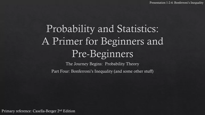
Primary reference: Casella-Berger 2 nd Edition Presentation 1-2- 4: - PowerPoint PPT Presentation

Presentation 1-2- 4: Bonferroni’s Inequality Primary reference: Casella-Berger 2 nd Edition

Presentation 1-2- 4: Bonferroni’s Inequality 𝑄 𝐵 ∪ 𝐶 = 𝑄 𝐵 + 𝑄(𝐶) − 𝑄(𝐵 ∩ 𝐶) Well, there’s one more interesting thing we can do with this. Remember that 𝑄 𝐵 ∪ 𝐶 ≤ 1 . The probability of an event can’t be greater than 1, after all. So let’s take this pretty self -evident bit of knowledge and do some tinkering: 𝑄 𝐵 ∪ 𝐶 = 𝑄 𝐵 + 𝑄(𝐶) − 𝑄(𝐵 ∩ 𝐶) ≤ 1 ⇒ 𝑄 𝐵 + 𝑄 𝐶 − 1 ≤ 𝑄 𝐵 ∩ 𝐶 ⇒ 𝑸 𝑩 ∩ 𝑪 ≥ 𝑸 𝑩 + 𝑸 𝑪 − 𝟐

Presentation 1-2- 4: Bonferroni’s Inequality 𝑸 𝑩 ∩ 𝑪 ≥ 𝑸 𝑩 + 𝑸 𝑪 − 𝟐 Simplified: The probability that two events will both happen is at least as high as the probability of the first event plus the probability of the second event minus 1.

Presentation 1-2- 4: Bonferroni’s Inequality 1 2 3 4 5 6 7 8 9 Behind six of these curtains is a brand-new car! Behind five of these curtains is a deadly snake. You get to choose one. What’s the probability of winning a brand-new car with a snake inside? …well, we can’t really say from the given information, but Bonferroni’s inequality can give us a lower bound for that probability.

Presentation 1-2- 4: Bonferroni’s Inequality 1 2 3 4 5 6 7 8 9 𝑸 𝑩 ∩ 𝑪 ≥ 𝑸 𝑩 + 𝑸 𝑪 − 𝟐 ⇒ 𝑸 ∩ ≥ 𝑸( ) + 𝑸( ) − 𝟐 ≥ 𝟕 𝟘 + 𝟔 𝟘 − 𝟐 = 𝟑 ⇒ 𝑸 ∩ 𝟘 The probability you’ll get a car with a snake inside is at least 2/9. Makes sense: with 6 cars, 5 snakes, and only 9 curtains, at least two curtains must be hiding both. Drive safe!

Presentation 1-2- 4: Bonferroni’s Inequality If some events 𝐷 1 , 𝐷 2 ,… form a partition (remember, that means that they don’t have any outcomes in common, but when combined, they have every outcome in the whole sample space Ω ), then: ∞ 𝑄 𝐵 = ෍ 𝑄(𝐵 ∩ 𝐷 𝑗 ) 𝑗=1

Presentation 1-2- 4: Bonferroni’s Inequality We’re not going to prove this (you’re welcome), but a diagram illustrates this pretty well. Let Ω be this rectangle, partitioned by 𝐷 1 , 𝐷 2 , 𝐷 3 , 𝐷 4 . Imagine that the probability of an event is the fraction of the rectangle that it occupies. That oval in the middle is A. Notice how A is comprised of its intersections with the C events? 𝐷 1 𝐷 2 𝐷 3 𝐷 4

Presentation 1-2- 4: Bonferroni’s Inequality For any set of events 𝐵 1 , 𝐵 2 ,… ∞ ∞ 𝑄 ራ 𝐵 𝑗 ≤ ෍ 𝑄(𝐵 𝑗 ) 𝑗=1 𝑗=1 So the probability of the union of these events is always less than or equal to the sum of the individual events’ probabilities. It’s a little more abstract than the last one, but another diagram should make it clear. 8

Presentation 1-2- 4: Bonferroni’s Inequality Again let Ω be this rectangle, with events 𝐵 1 , 𝐵 2 , 𝐵 3 . Imagine one more time that the probability of an event is the fraction of the rectangle that it occupies. If the three sets are totally disjoint, the probability of their union is equal to the sum of their probabilities: 𝐵 2 𝐵 1 𝐵 3

Presentation 1-2- 4: Bonferroni’s Inequality But now, they’re overlapping, so together, they take up less of the rectangle, and thus, in our analogy, the probability of their union is less than the sum of their individual probabilities. The probability of their union was at its maximum when they weren’t overlapping at all. 𝐵 3 𝐵 1 𝐵 2