Preview Videos Vis 97: Visualization of Music (video) 2/20/2014 - PDF document
2/20/2014 Comp/Phys/APSc 715 Multivariate & Ensemble Visualization Techniques 2/20/2014 Multivariate Comp/Phys/APSc 715 Taylor 1 Preview Videos Vis 97: Visualization of Music (video) 2/20/2014 Multivariate Comp/Phys/APSc 715
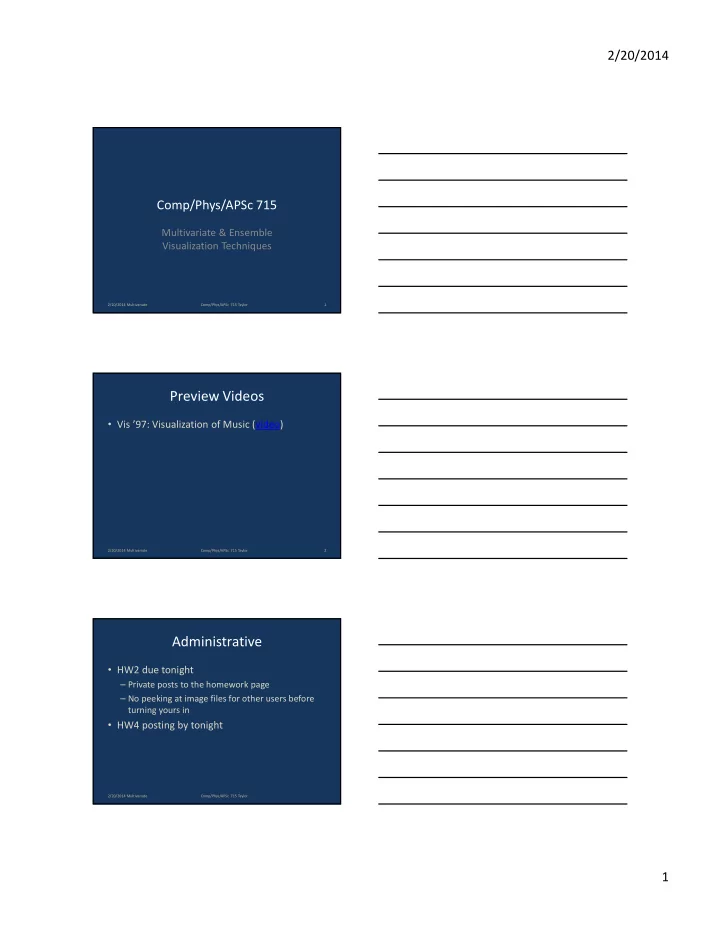
2/20/2014 Comp/Phys/APSc 715 Multivariate & Ensemble Visualization Techniques 2/20/2014 Multivariate Comp/Phys/APSc 715 Taylor 1 Preview Videos • Vis ’97: Visualization of Music (video) 2/20/2014 Multivariate Comp/Phys/APSc 715 Taylor 2 Administrative • HW2 due tonight – Private posts to the homework page – No peeking at image files for other users before turning yours in • HW4 posting by tonight 2/20/2014 Multivariate Comp/Phys/APSc 715 Taylor 1
2/20/2014 Team Dynamics • Working in teams is… – Good, because you can do more work – Hard, because of scheduling, communication, expectation management • Scheduling: Right After Class Find Partner • Communications/Expectation Management – Default: Work together on this at the same time – Clearly split the work and provide hard deadlines – Everyone participates equally: one member is not supposed to be doing all the work 2/20/2014 Multivariate Comp/Phys/APSc 715 Taylor 4 2/20/2014 Multivariate Comp/Phys/APSc 715 Taylor 5 Multivariate Data Display • At the frontier of data visualization • More art than science – Several combinations can show 2-3 data sets – Attempting combinations beyond this is difficult • Perceptual studies can help predict effectiveness – Avoiding interfering techniques gets you further – Still need to try it out and see • Easier in 2D than 3D • Several techniques shown today, some with characteristics listed 2/20/2014 Multivariate Comp/Phys/APSc 715 Taylor 6 2
2/20/2014 Multivariate Display Techniques • Glyphs • Heterogeneous Techniques • Texture • Layering/Subdividing Data Reduction • 2/20/2014 Multivariate Comp/Phys/APSc 715 Taylor 7 2/20/2014 Multivariate Comp/Phys/APSc 715 Taylor 8 Glyphs • Single graphical icon displaying multiple variables – Shape, color, other features • Designed for discrete, non-spatial data • Can be used to display fields – Scatter within 2D or 3D space – Display local characteristics 2/20/2014 Multivariate Comp/Phys/APSc 715 Taylor 9 3
2/20/2014 Classical Glyphs: Chernoff Faces 2/20/2014 Multivariate Comp/Phys/APSc 715 Taylor 10 Glyph Techniques Stick hard to use • Paul Ferry, SKIGRAPH ’99 – Profile Icon, Star Icon, Stick figure Icon • Ware – Probably only 3-4 distinguishable orientations – Don’t use parallel ones (as the figure on the right above does) – Varying color polarity adds more – Varying line width adds more 2/20/2014 Multivariate Comp/Phys/APSc 715 Taylor 11 Glyphs: Color + Size Vary 2/20/2014 Multivariate Comp/Phys/APSc 715 Taylor 12 4
2/20/2014 Glyph: Flow Probe • Wijk, J.J. van, A.J.S. Hin, W.C. deLeeuw, F.H. Post, “Three Ways to Show 3D Fluid Flow.” IEEE Computer Graphics and Applications, vol. 14, no. 5, p. 33-39, September 1994. 2/20/2014 Multivariate Comp/Phys/APSc 715 Taylor 13 Characteristics of Glyphs • Preattentive detection rules from before apply – size, orientation, and color coding • Integral vs. Separable dimensions – Integral dimensions are perceived holistically (upper) – Separable dimensions perceived independently (lower) 2/20/2014 Multivariate Comp/Phys/APSc 715 Taylor 14 • Attributes: • Sirens’ Song: 2/20/2014 Multivariate Comp/Phys/APSc 715 Taylor 15 5
2/20/2014 Number of Displayable Values • Many dimensions not independent – Texture relies on at least one color difference – Blinking and motion coding will interfere – Fortunate if you can display 8-dimensional data with color, shape, spatial position (not for glyphs in space), and motion. • Number of resolvable steps in each dimension – Maybe 4 values for each – Disallowing conjunction searches leaves 32 alternatives • ~4 values for each of 8 channels – 6 in spatial data – We didn’t see more than 3 work together at high density when doing combinations of different techniques 2/20/2014 Multivariate Comp/Phys/APSc 715 Taylor 16 2/20/2014 Multivariate Comp/Phys/APSc 715 Taylor 17 Heterogeneous Techniques • “Wandering in the desert” – “Simpleton” ideas prove their worth • Throw a bunch of techniques together • Hope for the best – Works okay for a few data sets – We found it hopeless for large numbers of sets 2/20/2014 Multivariate Comp/Phys/APSc 715 Taylor 18 6
2/20/2014 Heterogeneous 2D: Location + Width + Color 2/20/2014 Multivariate Comp/Phys/APSc 715 Taylor 19 UNC Nanoscience Heterogeneous 2D: Height + Texture 2/20/2014 Multivariate Comp/Phys/APSc 715 Taylor 20 UNC Nanoscience Heterogeneous 2D: Height + Color + Contour Non-isoluminant color 2/20/2014 Multivariate Comp/Phys/APSc 715 Taylor 21 7
2/20/2014 UNC Nanoscience Heterogeneous 2D: Color + Texture + Bump Tex 2/20/2014 Multivariate Comp/Phys/APSc 715 Taylor 22 UNC Nanoscience Heterogeneous 2D • Promise – 1 Height dimension, 2 Color dimensions, 3+ Texture dimensions = 6+ perceptual dimensions • Results – Luminance contrast in color confounds shape – High-frequency components of texture confound color – Multiple textures confound each other 2/20/2014 Multivariate Comp/Phys/APSc 715 Taylor 23 Heterogeneous 2D: Height + Color + Glyph • Haber, Koh, Lee – UIUC • Found in – Keller & Keller p. 62 Rainbow 2/20/2014 Multivariate Comp/Phys/APSc 715 Taylor 24 8
2/20/2014 Heterogeneous 3D: Slice + Contour + Color + Tex. 2/20/2014 Multivariate Comp/Phys/APSc 715 Taylor 25 Heterogeneous 3D: Surface + Color + Texture • Vis 2001: Severance, Lazos, Keefe, “Wind Tunnel Data Fusion and Immersive Visualization” Rainbow 2/20/2014 Multivariate Comp/Phys/APSc 715 Taylor 26 2/20/2014 Multivariate Comp/Phys/APSc 715 Taylor 27 9
2/20/2014 Texture-Based Multivariate 2D • Varying several characteristics to display data – Adjusting size, density, and regularity – Adjusting size, orientation, and density – Adjusting scale, orientation, and contrast – Spot Noise: Adjusting orientation and hue/saturation • Varying a single characteristic to differentiate between multiple layers, intensity in each layer (both texturing and layering technique) – Beyond four scalar fields in the same image – Oriented Slivers – Data-Driven Spots 2/20/2014 Multivariate Comp/Phys/APSc 715 Taylor 28 Texture Dimensions • Chris Healey • Height = cultivation level • Density = ground type – Sparse = alluvial – Dense = wetland • Grayscale = vegetation – Dark = plains – Light = forest – White = woodland 2/20/2014 Multivariate Comp/Phys/APSc 715 Taylor 29 Chris Healey: Size, Density, Regularity, Hue Sort of like glyphs + arrangement Result is ~texture 2/20/2014 Multivariate Comp/Phys/APSc 715 Taylor 30 10
2/20/2014 Chris Healey: Size, Density, Orientation, Color Dense glyphs form a texture 2/20/2014 Multivariate Comp/Phys/APSc 715 Taylor 31 Texture: Spot Noise • Invented by JJ van Wijk, SIGGRAPH 1991 – Spot orientation, spot size, hue – Can vary scale – Can vary shape • Affects texture Rainbow 2/20/2014 Multivariate Comp/Phys/APSc 715 Taylor 32 Quantitative Texton Sequences for Bivariate Maps (Ware) 2/20/2014 Multivariate Comp/Phys/APSc 715 Taylor 33 11
2/20/2014 2/20/2014 Multivariate Comp/Phys/APSc 715 Taylor 34 Layer-Based Multivariate 2D • Subdividing the surface • Varying a single characteristic to differentiate between multiple layers, intensity in each layer (both texturing and layering technique) – Beyond four scalar fields in the same image – Oriented Slivers – Data-Driven Spots – Nested and intersecting surfaces • Layering heterogeneous techniques – Crawfis – Laidlaw – Urness/Interrante 2/20/2014 Multivariate Comp/Phys/APSc 715 Taylor 35 Attribute Blocks: Visualizing Multiple Continuously Defined Attributes (James Miller) Cyan isoluminant with background 2/20/2014 Multivariate Comp/Phys/APSc 715 Taylor 36 12
2/20/2014 Multivariate Visualization on Parametric Surfaces (James Miller) 2/20/2014 Multivariate Comp/Phys/APSc 715 Taylor 37 Multivariate Visualization on Parametric Surfaces (James Miller) 2/20/2014 Multivariate Comp/Phys/APSc 715 Taylor 38 Visualizing Multidimensional Scalar Data Using Hexagonal Tiles (Ramachandran and Healey) New Mexico State Employment Affluence Bachelor’s degree level Income 2/20/2014 Multivariate Comp/Phys/APSc 715 Taylor 39 13
2/20/2014 Visualizing Multidimensional Scalar Data Using Hexagonal Tiles (Ramachandran and Healey) 2/20/2014 Multivariate Comp/Phys/APSc 715 Taylor 40 Chris Weigle, UNC Oriented Slivers: Four Tube Orientations • Four scalar fields – Here, 4 orientations – Each mapped to displayed orientation • Overall intensity shows total amount of material 2/20/2014 Multivariate Comp/Phys/APSc 715 Taylor 41 Chris Weigle, UNC Oriented Slivers • Background color shows another data set – Reveals dark slivers – Shows region boundary • Close-up of 3 data sets 2/20/2014 Multivariate Comp/Phys/APSc 715 Taylor 42 14
Recommend
More recommend
Explore More Topics
Stay informed with curated content and fresh updates.
