Predictor-corrector ensemble filters for high-dimensional nonlinear - PowerPoint PPT Presentation

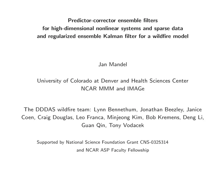
Predictor-corrector ensemble filters for high-dimensional nonlinear systems and sparse data and regularized ensemble Kalman filter for a wildfire model Jan Mandel University of Colorado at Denver and Health Sciences Center NCAR MMM and IMAGe The DDDAS wildfire team: Lynn Bennethum, Jonathan Beezley, Janice Coen, Craig Douglas, Leo Franca, Minjeong Kim, Bob Kremens, Deng Li, Guan Qin, Tony Vodacek Supported by National Science Foundation Grant CNS-0325314 and NCAR ASP Faculty Fellowship

The challenge: data assimilation into highly nonlinear wildfire models Simulation code is a black box ⇒ ensemble filters • Highly non-gaussian ⇒ predictor-corrector ensemble filters Jan Mandel and Jonathan Beezley, CCM Report 232, 2006 • Need to avoid nonphysical solutions ⇒ regularized EnKF C. J. Johns and J. Mandel, CCM Report 221, 2005; Env. Ecol. Stat., to appear • Efficient parallel EnKF for large data Jan Mandel, CCM Report 231, 2006 • Data assimilation into a one-step reaction-diffusion fire model Jan Mandel, Lynn S. Bennethum, Jonathan Beezley, Janice L. Coen, Craig C. Douglas, Leopoldo P. Franca, Minjeong Kim, and Anthony Vodacek, CCM Report 233, 2006 http://www-math.cudenver.edu/ccm/reports

Data Assimilation: Sequential Statistical Estimation State of the model is probability density p ( u ) of the system state u Analysis cycle: = ⇒ = ⇒ p a,t k − 1 p f,t k p a,t k advance Bayes p f,t k : “forecast” probability density at time t k p a,t k : “analysis” probability density at time t k Model advanced in time by the model At analysis time , new data incorporated by the use of Bayes theorem p a,t k ( u ) ∝ p ( d | u ) p f,t k ( u ) � pdν = 1; ν is some ∝ means proportional; densities are always scaled so that underlying measure (Lebesgue in finite dimension). p ( d | u ) is data likelihood = probability density that the data value is d if the system state is u

Data Likelihood data likelihood = probability density that the data value is d if the system state is u Data likelihood can be obtained from data error probability density p ε (assumed known) and observation function h ( u )=what the data would be if there are no errors and the system state is u : P ( d − h ( u ) ∈ A ) = � A p ε dν ⇒ p ( d | u ) = p ε ( d − h ( u )) This formula tacitly assumes that data error is additive and it does not depend on d and u . All data must be accompanied by an error estimate (=error probability distribution) otherwise it is meaningless.

Ensemble Approach Model state (= probability density of the system state) is represented by a weighted ensemble ( u k , w k ), k = 1 , . . . , N N u k are system state vectors, w k are positive weights, w k = 1. � k =1 Simple case: all weights are same w k = 1 /N , { u k } is a sample from model state p, u k ∼ p (values of independent identically distributed random variables with density p )

Weighted ensemble How to represent a probability density by the weights of an ensemble? Ensemble members are a sample from some probability density, u k ∼ p π . We want the weighted ensemble represent another probability density p . For given function f , consider Monte-Carlo approximation of the integral N Ω f p � � � Ω fpdν = p π dν ≈ w k f ( u k ) p π k =1 p ( u k ) with the weights w k = 1 p π ( u k ) . N So, given a sample { u k } from p π , w k ∝ p ( u k ) p ∼ ( u k , w k ) , p π ( u k ) , u k ∼ p π

Sequential Importance Sampling (SIS) a.k.a. Sequential Monte Carlo (SMC) a.k.a. Particle Filters (PF) Given forecast ensemble p f ∼ ( u f k , w f k ) � � u a Given sample from proposal density ∼ p π k Apply Bayes theorem: p a ( u ) = p ( u | d ) ∝ p ( d | u ) p f ( u ) = ⇒ � � u a k ∝ p a ( u a p f k ) k ( u a k , w a w a k ) ∝ p ( d | u a k ) ∼ p a , k ) p π ( u a � � u a p π k k = u f SIS chooses u a k (does not change the ensemble) and only updates the k ∝ p f ( u k ) u f ∼ p π , w f � � weights = ⇒ already p π ( u k ) = ⇒ k d | u f w f � � w a k ∝ p k k

Sequential Importance Sampling with Resampling (SIR) Trouble with SIS: 1. data likelihoods can be very small, then 2. the analysis ensemble represents the analysis density poorly 3. one or a few of the analysis weights will dominate Standard solution: SIR (Gordon 1993,...) 1. Resample by choosing u a k with probability ∝ w a k , set all weights equal 2. rely on stochastic behavior of the model to recover spread. But there is still trouble: 1. huge ensembles (thousands) are needed because the analysis distribution is effectively approximated only by those ensemble members that have large weights, and a vast majority of weights is infinitesimal 2. if the model is not stochastic, need artificial perturbation to recover ensemble spread Solution: Predictor-corrector filters (new) Place the analysis ensemble so that the weights are all reasonably large .

Predictor-Corrector Filters (new) Given forecast ensemble and a proposal ensemble obtained by a predictor p f ∼ ( u f ℓ , w f p π ∼ ( u a ℓ ) , k ) , Apply Bayes theorem: p a ( u ) = p ( u | d ) ∝ p ( d | u ) p f ( u ) = ⇒ � � u a k ∝ p a ( u a p f k ) k ( u a k , w a w a k ) ∝ p ( d | u a k ) ∼ p a , k ) p π ( u a � � u a p π k Estimate the ratio of densities from ( u f k , w f k ) to get the analysis weights ( corrector ): e k ≈ p f ( u a k ) d | u f � � � � w a ew a d | u a k ∝ p k ∝ p e k , k k p π ( u a k ) Trouble: 1. density estimates in high dimension are intractable 2. need to estimate far away from and outside of the span of the sample Solution: 1. the probability densities are not arbitrary: they come from probability measures on spaces of smooth functions, low effective dimension 2. nonparametric estimation that depends only the concept of distance

Nonparametric Density Estimation Let { u ℓ : ℓ = 1 , . . . , N } ∼ p and B h ( x ) = { y : � y − x � < h } be the ball with radius h and center x . The density estimate p N,h ( y ) = number of u ℓ ∈ B h ( x ) → p ( y ) in probability N measure of B h ( x ) if p is continuous at y and h = h ( N ) is the distance to k ( N )-th nearest u k from y k ( N ) → ∞ , k ( N ) /N → 0 , N → ∞ (Loftsgaarden-Quesenberry (1965) in R n and Lebesgue measure), or h = h ( N ) → 0 , N measure of B h ( x ) → 0 , N → ∞ (Rosenblatt (1956) in R n , Dabo-Niang (2004) in Banach spaces)

Nonparametric Estimation of Importance Weights e k ≈ p f ( u a k ) � � Recall the analysis weights: w a d | u a k ∝ p e k , k p π ( u a k ) Generalize density estimation to weighted ensemble: � w ℓ ℓ : � u ℓ − x � <h ( u k , w k ) ∼ p, measure of B h ( x ) ≈ p ( x ) Recall forecast ensemble ( u f k , w f k ) N k =1 and proposal ensemble ( u a k ) N k =1 Substitute and the (generally unknown) measure of B h ( x ) falls out: � <h w f � � � � � u a � u f ℓ ℓ − u a p f ℓ : � � k k � ≈ 1 � u a � p π � � � u f N k ℓ − u a ℓ : � <h � � k It remains to choose the norm �·� in the estimate. The bandwidth is chosen as on the previous page.

Choosing the norm in density ratio estimate Need performance independent of dimension = ⇒ use infinite dimension, model state is probability distribution on a space of functions The densities p f , p a , p π need to exist w.r.t. some underlying measure ν . The ratio of densities p f /p π does not depend on ν as long as the densities exist and are nonzero but the estimate does . The measure ν is linked to the norm via the measure of the ball, ν ( B h ( x )), need B h ( x ) > 0 and lim h → 0 ν ( B h ( x )) = 0. The density of probability distribution ϕ of system state w.r.t. ν exists ⇐ ⇒ ∀ A : v ( A ) = 0 = ⇒ ϕ ( A ) = 0 (Radon-Nikodym theorem)

Choosing the norm in density ratio estimate (translation) The norm is linked to the underlying measure via the measure of small balls, which need to have reasonable properties. The probability for a function in the state space to fall into a ball should be positive and have limit zero for small balls. The probability for a function in the state space to fall in a set of measure ν zero should be zero. In infinite dimension, this is far from automatic, and restricts the choice of the norm in the density estimate! Lebesgue measure in infinite dimension does not exist = ⇒ use gaussian measure At least the initial ensemble should be from probability distribution that has density w.r.t. the measure ν .

Smooth random fields The initial ensemble is constructed by a perturbation of initial condition by smooth random fields; this gives the underlying measure ν and associated norm Random smooth function (random field) from some space V ∞ � u ( x ) = λ n v n e n ( x ) , ν n ∼ N (0 , 1) n =1 { e n } is Fourier basis of V , 1D example: e n ( x ) = sin ( nx ) λ n > 0, λ n − → 0 determine smoothness: faster decay of λ n = ⇒ smoother u Well known in geosciences as “random fields by FFT” (Evensen 1994,...). λ n and e n are eigenvalues and eigenvectors of the covariance of the random field. Theory of gaussian measures: must assume � ∞ n =1 λ 2 n < ∞ .