Pr Proba obability a and nd Sta Statistics Basic c concepts - PowerPoint PPT Presentation
Pr Proba obability a and nd Sta Statistics Basic c concepts pts (from a a physi sicist st p point of vi view) Benoi noit C t CLEMENT Univer ersit t J J. Four urier er / / L LPSC bclem ement@l nt@lpsc.in2p n2p3.fr
Pr Proba obability a and nd Sta Statistics Basic c concepts pts (from a a physi sicist st p point of vi view) Benoi noit C t CLEMENT – Univer ersité té J J. Four urier er / / L LPSC bclem ement@l nt@lpsc.in2p n2p3.fr
Bibliography Kendall’s Advanced theory of statistics, Hodder Arnold Pub. volume 1 : Distribution theory, A. Stuart et K. Ord volume 2a : Classical Inference and and the Linear Model, A. Stuart, K. Ord, S. Arnold volume 2b : Bayesian inference, A. O’Hagan, J. Forster The Review of Particle Physics, K. Nakamura et al., J. Phys. G 37, 075021 (2010) (+Booklet) Data Analysis: A Bayesian Tutorial, D. Sivia and J. Skilling, Oxford Science Publication Statistical Data Analysis, Glen Cowan, Oxford Science Publication Analyse statistique des données expérimentales, K. Protassov, EDP sciences Probabilités, analyse des données et statistiques, G. Saporta, Technip Analyse de données en sciences expérimentales, B.C., Dunod 2
Sample and population POPULATION SAMPLE Potentially infinite Finite size size Selected through a random proces cess eg. All possible eg. Result of a results measurement Characterizing the sample, the population and the sampling process Pr Probabi bility th theory (first lecture) 3
Statistics PH PHYSI SICS eters θ param ameter Observ rvab able POPULATION SAMPLE x; θ ) f(x; IN INFEREN ENCE Finite size x i EX EXPER PERIMENT Using the sample to estimate the characteristics of the population Stati tisti tical cal i infer erence ence (second lecture) 4
Random process A random process (« measurement » or « experiment ») is a process whose outcom tcome c e cannot nnot be pred edicted cted w with c th certa tainty nty. It will be described by : Unive verse se: Ω = = set of all possible outc outcomes. Eve Event : log ogical cond condition on an on an out outcome. It can either be true or false; an event splits the universe in 2 subsets. An event A will be identified by the subset A for which A is true. 5
Probability A prob obab ability ty f funct nction on P is defined by : (Kolmogorov, 1933) P : : {Events ents} → [0: [0:1] A A → P(A) A) satisfying : P( P( Ω )=1 =1 P(A (A or or B) B) = P P(A (A) + P P(B) (B) i if A A and and B B = Ø Ø Inter terpret etati ation o on of t this n number er : : - Freq eque uenti ntist approach ach : if we repeat the random process a great number of times n , and count the number of times the outcome satisfy event A, n A then the ratio : n lim P(A) A = defines a probability n n → +∞ - Bayes esian an i inter erpreta etati tion on : a probability is a measure of 6 the credibility associated to the event.
Simple logic Event « not A not A » » is associated with the complement A. P(A) (A) = = 1–P(A) (A) P( P(Ø) = ) = 1-P( P( Ω ) = ) = 0 Event « A A and and B B » » Event « A A or or B B » » P(A (A or B B) = P(A)+ A)+P(B) (B)–P(A and and B) B) 7
Conditional probability If an event B B is kno nown to b to be tr e true, one can restrain the universe to Ω ’=B and define a new probability function on this universe, the condit itio ional p l probabilit ility. P(A|B) = B) = « probability ty o of A A given B en B » P(A and B) = P(A | B) P(B) The definition of conditional probability leads to : P(A and B) = P(A|B).P(B) = P(B|A).P(A) Hence relating P(A|B) to P(B|A) by the Bayes es t theor eorem em : : P(A | B).P(B) = P(B | A) 8 P(A)
Incompatibility and Indpendance Two incompa pati tibl ble events cannot be true simultaneously, then : P(A P(A a and B B) = ) = 0 0 P(A P(A or B B) = ) = P(A (A)+ )+P( P(B) B) Two events are indepe pende dent, if the realization of one is not linked in any way to the realization of the other : P(A P(A|B |B)=P(A) P(A) and P(B P(B|A) = |A) = P(B P(B) P(A P(A and B B) ) = P(A P(A). ).P( P(B) B) 9
Random variable When the outcome of the random process is a num number (real or integer), we associate to the random process a rand ndom om v variab able X e X. Each realization of the process leads to a particular result : X= X=x. x x is a realization of X. X. For a discr crete v te variab able : Probabilit lity l law : p(x) = ) = P(X= X=x) For a real v l varia iable le : P(X=x)=0, Cumul ulat ative d e dens nsity ty f functi nction on : F(x F(x) = = P(X (X<x) dF = F(x+dx)-F(x) = P(X < x+dx) - P(X < x) = P(X < x or x < X < x+dx) - P(X < x) = P(X < x) + P(x < X < x+dx) - P(X < x) = P(x < P(x < X < x+d +dx) = ) = f(x) (x)dx dF f(x) = Probability ty d density ty f functi nction ( on (pdf) : : 10 dx
Density function Probab ability ty d density ty f functi ction Cumulati ative e density ty f functi ction F(x) f(x) 1 +∞ x x ∫ f(x)dx P( Ω ) 1 = = By construction : − ∞ F(- ) P(Ø) 0 ∞ = = Note : discrete variables can also be described by a F( ) P( Ω ) 1 +∞ = = probability density function a using Dirac distributions: ∫ F(a) f(x)dx = ∑ f(x) p(i) δ(i - x) = - ∞ b i ∫ P(a X b) F(b) - F(a) f(x)dx < < = = ∑ p(i) 1 = 11 a i
Moments For any function g( g(x), the expectati ectation of g is : ∫ E[g(X)] g(x)f(x)dx = It’s the mean value of g Momen ents ts μ k are the expectation of X k . 0 th moment : μ 0 =1 =1 (pdf normalization) 1 st moment : μ 1 = μ (mean) X’ = ’ = X- μ 1 is a central tral v vari riab able 2 nd central moment : μ ’ 2 = σ 2 (variance) ∫ (t) E[e ixt ] f(x)e ixt dx FT 1 [f] ϕ = = = − Characteri racteristic f c functi ction : (itx) k (it) k ∫∑ ∑ (t) f(x)dx μ From Taylor expansion : ϕ = = k k! k! k k d k ϕ Pdf entirely defined by its moments μ i k = − k dt k CF : useful tool for demonstrations 12 t 0 =
Sample PDF A sample ple is obtained from a random d om drawi wing ng within a populati ation, described by a probability density function. We’re going to discuss how to charact aracteri erize, e, indep epen enden entl tly fro rom one e an anoth ther: : - a populati ation - a sample ple To this end, it is useful, to consider a sample as a finite set from which one can randomly draw elements, with equipropability We can the associate to this process a probability density, the empiri rical al density ty or sample e density ty 1 ∑ f (x) δ(x - i) = sample n i This density will be useful to translate properties of 13 distribution to a finite sample.
Characterizing a distribution How t to reduce a uce a distr tributi ution/ on/sam ample t e to a fini nite te num number of of val alues ? ? Meas asur ure o e of l locat ation on: Reducing the distribution to one c e centr ntral al v value ue -> Res Result Meas asur ure o e of d disper ersion on: Spread ad of the distribution around the central value -> Uncer ertai tainty nty/Error Freq equen uency cy t table/ e/hi histo togram am (for a finite sample) 14
Location and dispersion sample (size n ) population Mean val Mea alue : Sum (integral) of all possible values weighted by the probability of occurrence: 1 n ∑ +∞ μ x x ∫ μ x xf(x)dx = = = = i n − ∞ i 1 = sample (size n ) population Standard ard d deviati ation ( σ ) and vari rian ance ce (v= σ ²) ²) : Mean value of the squared deviation to the mean : 2 ∫ 1 n ∑ v σ (x μ) 2 2 v σ (x μ ) f(x)dx 2 = = − = = − i n i 1 = Koen enig’s th theo eorem : ∫ ∫ ∫ σ 2 x 2 f(x)dx μ 2 f(x)dx 2 μ xf(x)dx x 2 μ 2 x 2 x 2 = + − = − = − 15
Discrete distributions Binomial al distri ributi tion: randomly choosing K objects within a finite set of n, with a fixed drawing probability of p Variable : K Parameters : n,p ,p p = 0.65 n! n = 10 P(k;n, p) p k (1 p) n k Law : = − − k! (n k)! − Mean : np np Variance : np( p(1-p) p) Poisson d distri tributi tion : limit of the binomial when n →+ ∞,p → 0,np= p= λ Counting events with fixed probability per time/space unit. Variable : K λ = 6.5 Parameters : λ e λ - λ k P(k; λ) = Law : k! Mean : λ Variance : λ 16
Real distributions Uniform rm d distri ributi tion : equiprobability over a finite range [a,b] Parameters : a,b ,b 1 f(x; a,b) if a x b Law : = < < b a − μ (a b)/2 = + Mean : v σ 2 (b a) 2 /12 = = − Variance : Normal al d distri tributi tion (Gaussian an) ) : limit of many processes Parameters : μ , , σ 2 (x μ) − 1 − f(x; μ, σ) e 2 = 2 σ Law : σ 2 π Chi hi-square d are distri tributi tion : sum of the square of n normal reduced variables 2 X - μ n ∑ Variable : k X C = k σ k 1 Parameters : n = X k n c n n 1 1 − − − f(c;n) c e 2 Γ Law : = 2 2 2 2 17 Mean : n n Variance : 2n 2n
Convergence 18
Recommend
More recommend
Explore More Topics
Stay informed with curated content and fresh updates.
