Power variation and p -variation of sample functions of stochastic - - PowerPoint PPT Presentation

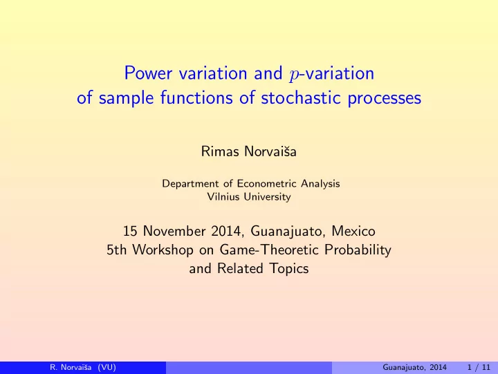
Power variation and p-variation

• f sample functions of stochastic processes

Rimas Norvaiˇ sa

Department of Econometric Analysis Vilnius University

15 November 2014, Guanajuato, Mexico 5th Workshop on Game-Theoretic Probability and Related Topics

• R. Norvaiˇ

sa (VU) Guanajuato, 2014 1 / 11

Power variation of a function

Let f be a regulated function on [0, T], i.e. there exist limits f(t−) := lim

x↑t f(x)

and f(s+) := lim

x↓s f(x)

for each 0 ≤ s < t ≤ T. Let λ = {λn : n ≥ 1} be a nested sequence of partitions λn = (tn

i )m(n) i=0

• f

[0, T] such that ∪nλn is dense in [0, T]. Let 1 ≤ p < ∞. We say that f has p-th power λ-variation on [0, T], if there is a regulated function V on [0, T] such that V (0) = 0 and for each 0 ≤ s < t ≤ T V (t) − V (s) = lim

n→∞ m(n)

• i=1

|f((tn

i ∧ t) ∨ s) − f((tn i−1 ∧ t) ∨ s))|p,

V (t) − V (t−) = |f(t) − f(t−)|p and V (s+) − V (s) = |f(s+) − f(s)|p.

• R. Norvaiˇ

sa (VU) Guanajuato, 2014 2 / 11

p-variation of a function

Let f be a function on [0, T] (must be regulated if it has bounded p-variation defined next). Let 1 ≤ p < ∞. The p-variation of f is the quantity vp(f, [0, T]) defined to be sup n

• i=1

|f(ti) − f(ti−1)|p : (ti)n

i=0 is a partition of [0, T]

• ,

which may be finite or infinite. If vp(f, [0, T]) < ∞ then one says that f has bounded p-variation. The p-variation index of f is the quantity υ(f, [0, T]) defined to be inf{p ≥ 1: vp(f, [0, T]) < ∞}. if the set is non-empty and defined to be +∞ otherwise.

• R. Norvaiˇ

sa (VU) Guanajuato, 2014 3 / 11

Example: Wiener process

Let W = {W(t): t ∈ [0, T]} be a standard Wiener process. Due to results of N. Wiener (1923) and P. L´ evy (1940): vp(W, [0, T]) < +∞ a.s. iff p > 2, and v2(W, [0, T]) = +∞ a.s. Thus the p-variation index υ(W, [0, T]) = 2 a.s. More precise information can be obtained in terms of φ-variation, defined as p-variation except that the power function x → xp, x ≥ 0, is replaced by a function φ.

• S. J. Taylor (1972): vψ1(W, [0, T]) < +∞ a. s., where

ψ1(x) := x2/LL(1/x), 0 < x ≤ e−e. Also, vψ(W) = +∞ a.s. for any ψ such that ψ1(x) = o(ψ(x)) as x ↓ 0.

• R. Norvaiˇ

sa (VU) Guanajuato, 2014 4 / 11

Example: Wiener process

Let W = {W(t): t ∈ [0, T]} be a standard Wiener process. Due to results of N. Wiener (1923) and P. L´ evy (1940): vp(W, [0, T]) < +∞ a.s. iff p > 2, and v2(W, [0, T]) = +∞ a.s. Thus the p-variation index υ(W, [0, T]) = 2 a.s. More precise information can be obtained in terms of φ-variation, defined as p-variation except that the power function x → xp, x ≥ 0, is replaced by a function φ.

• S. J. Taylor (1972): vψ1(W, [0, T]) < +∞ a. s., where

ψ1(x) := x2/LL(1/x), 0 < x ≤ e−e. Also, vψ(W) = +∞ a.s. for any ψ such that ψ1(x) = o(ψ(x)) as x ↓ 0.

• R. Norvaiˇ

sa (VU) Guanajuato, 2014 4 / 11

Example: Wiener process

Let W = {W(t): t ∈ [0, T]} be a standard Wiener process. Due to results of N. Wiener (1923) and P. L´ evy (1940): vp(W, [0, T]) < +∞ a.s. iff p > 2, and v2(W, [0, T]) = +∞ a.s. Thus the p-variation index υ(W, [0, T]) = 2 a.s. More precise information can be obtained in terms of φ-variation, defined as p-variation except that the power function x → xp, x ≥ 0, is replaced by a function φ.

• S. J. Taylor (1972): vψ1(W, [0, T]) < +∞ a. s., where

ψ1(x) := x2/LL(1/x), 0 < x ≤ e−e. Also, vψ(W) = +∞ a.s. for any ψ such that ψ1(x) = o(ψ(x)) as x ↓ 0.

• R. Norvaiˇ

sa (VU) Guanajuato, 2014 4 / 11

Example: fractional Brownian motion

Let BH = {BH(t): t ∈ [0, T]} be a fractional Brownian motion with the Hurst index H ∈ (0, 1), i.e. a Gaussian stochastic process with mean zero and the covariance function EBH(t)BH(s) = 1 2

• t2H + s2H − |t − s|2H

s, t ∈ [0, T]. Let λn = (tn

i )m(n) i=0 , n ∈ N, be a sequence of partitions of [0, T] such that

• maxi(tn

i − tn i−1)

1∧(2H) log n → 0 as n → ∞. Then a.s. lim

n→∞ m(n)

• i=1
• BH(tn

i ) − BH(tn i−1)

• 1/H = E|η|1/HT,

where η is a standard normal random variable. Thus, almost every sample function of BH has 1/H power λ-variation t → cHt, t ∈ [0, T]. Also, a.s. v1/H(BH, [0, T]) = +∞ and υ(BH, [0, T]) = 1/H.

• R. Norvaiˇ

sa (VU) Guanajuato, 2014 5 / 11

Weighted power variation for a Gaussian process

Let X = {X(t): t ∈ [0, T]} be a mean zero Gaussian process s.t. there is a real valued function ρ defined on [0, T] and ”equivalent” to h → (E[X(s + h) − X(s)]2)1/2 near zero uniformly in s ∈ [ǫ, T) for each ǫ > 0. If X has stationary increments, then one can take ρ(h) = (E[X(s + h) − X(s)]2)1/2. Under suitable hypotheses on the covariance of X and for a suitable set of positive r we proved that a.s. lim

n→∞ mn

• i=1

|X(tn

i ) − X(tn i−1)|r

[ρ(tn

i − tn i−1)]r

(tn

i − tn i−1) = E|η|rT,

(1) where η is a standard normal random variable, and ((tn

i )mn i=0) is a

sequence of partitions of [0, T] such that the mesh maxi(tn

i − tn i−1)

tends to zero as n → ∞ sufficiently fast.

• R. Norvaiˇ

sa (VU) Guanajuato, 2014 6 / 11

Weighted power variation for a Gaussian process

Let X = {X(t): t ∈ [0, T]} be a mean zero Gaussian process s.t. there is a real valued function ρ defined on [0, T] and ”equivalent” to h → (E[X(s + h) − X(s)]2)1/2 near zero uniformly in s ∈ [ǫ, T) for each ǫ > 0. If X has stationary increments, then one can take ρ(h) = (E[X(s + h) − X(s)]2)1/2. Under suitable hypotheses on the covariance of X and for a suitable set of positive r we proved that a.s. lim

n→∞ mn

• i=1

|X(tn

i ) − X(tn i−1)|r

[ρ(tn

i − tn i−1)]r

(tn

i − tn i−1) = E|η|rT,

(1) where η is a standard normal random variable, and ((tn

i )mn i=0) is a

sequence of partitions of [0, T] such that the mesh maxi(tn

i − tn i−1)

tends to zero as n → ∞ sufficiently fast.

• R. Norvaiˇ

sa (VU) Guanajuato, 2014 6 / 11

Partial sum process

Let X1, X2, . . . be real random variables. For each n = 1, 2, . . . , let Sn be the n-th partial sum process Sn(t) := X1 + · · · + X⌊tn⌋, t ∈ [0, 1], Thus for each n = 1, 2, . . . and t ∈ [0, 1], Sn(t) =        0, if t ∈ [0, 1/n), X1 + · · · + Xk, if t ∈ [ k

n, k+1 n ),

k ∈ {1, . . . , n − 1}, X1 + · · · + Xn, if t = 1. Then for any p ∈ (0, ∞), vp(Sn, [0, 1]) = max   

m

• j=1
• Xkj−1+1 + · · · + Xkj
• p

   , where the maximum is taken over 0 = k0 < · · · < km = n and 1 ≤ m ≤ n.

• R. Norvaiˇ

sa (VU) Guanajuato, 2014 7 / 11

Partial sum process

Let X1, X2, . . . be real random variables. For each n = 1, 2, . . . , let Sn be the n-th partial sum process Sn(t) := X1 + · · · + X⌊tn⌋, t ∈ [0, 1], Thus for each n = 1, 2, . . . and t ∈ [0, 1], Sn(t) =        0, if t ∈ [0, 1/n), X1 + · · · + Xk, if t ∈ [ k

n, k+1 n ),

k ∈ {1, . . . , n − 1}, X1 + · · · + Xn, if t = 1. Then for any p ∈ (0, ∞), vp(Sn, [0, 1]) = max   

m

• j=1
• Xkj−1+1 + · · · + Xkj
• p

   , where the maximum is taken over 0 = k0 < · · · < km = n and 1 ≤ m ≤ n.

• R. Norvaiˇ

sa (VU) Guanajuato, 2014 7 / 11

p-variation of partial sum process

• J. Bretagnolle (1972): given p ∈ (0, 2) there exists a finite constant

Cp such that n

• i=1

E|Xi|p ≤

• Evp(Sn) ≤ Cp

n

• i=1

E|Xi|p, provided X1, X2, . . . are independent, E|Xi|p < ∞ and EXi = 0 if p > 1. Suppose that X1, X2, . . . are independent identically distributed real random variables, EX1 = 0 and EX2

1 = 1. Let Lx := max{1, log x},

x > 0.

• J. Qian (1998): boundedness in probability

v2(Sn) = OP (nLLn) as n → ∞. Also, OP (nLLn) cannot be replaced by op(nLLn), if in addition E|X1|2+ǫ < ∞ for some ǫ > 0.

• R. Norvaiˇ

sa (VU) Guanajuato, 2014 8 / 11

p-variation of partial sum process

• J. Bretagnolle (1972): given p ∈ (0, 2) there exists a finite constant

Cp such that n

• i=1

E|Xi|p ≤

• Evp(Sn) ≤ Cp

n

• i=1

E|Xi|p, provided X1, X2, . . . are independent, E|Xi|p < ∞ and EXi = 0 if p > 1. Suppose that X1, X2, . . . are independent identically distributed real random variables, EX1 = 0 and EX2

1 = 1. Let Lx := max{1, log x},

x > 0.

• J. Qian (1998): boundedness in probability

v2(Sn) = OP (nLLn) as n → ∞. Also, OP (nLLn) cannot be replaced by op(nLLn), if in addition E|X1|2+ǫ < ∞ for some ǫ > 0.

• R. Norvaiˇ

sa (VU) Guanajuato, 2014 8 / 11

p-variation of partial sum process

• J. Bretagnolle (1972): given p ∈ (0, 2) there exists a finite constant

Cp such that n

• i=1

E|Xi|p ≤

• Evp(Sn) ≤ Cp

n

• i=1

E|Xi|p, provided X1, X2, . . . are independent, E|Xi|p < ∞ and EXi = 0 if p > 1. Suppose that X1, X2, . . . are independent identically distributed real random variables, EX1 = 0 and EX2

1 = 1. Let Lx := max{1, log x},

x > 0.

• J. Qian (1998): boundedness in probability

v2(Sn) = OP (nLLn) as n → ∞. Also, OP (nLLn) cannot be replaced by op(nLLn), if in addition E|X1|2+ǫ < ∞ for some ǫ > 0.

• R. Norvaiˇ

sa (VU) Guanajuato, 2014 8 / 11

p-variation of partial sum process

• R. Norvaiˇ

sa and A. Raˇ ckauskas (2008): Let X1, X2, . . . be a sequence of independent identically distributed random variables and let Sn be the n-th partial sum process. The convergence in law (in the sense of Hoffmann-Jørgensen) n−1/2Sn ⇒ σW in Wp[0, 1] as n → ∞ holds if and only if EX1 = 0 and σ2 := EX2

1 < ∞.

Here Wp[0, 1] is the Banach space of functions f on [0, 1] having bounded p-variation with respect to the norm f[p] := fsup,[0,1] + vp(f, [0, 1])1/p. In particular, the convergence in distribution n−p/2vp(Sn, [0, 1]) → σpvp(W, [0, 1]) as n → ∞ holds.

• R. Norvaiˇ

sa (VU) Guanajuato, 2014 9 / 11

p-variation of partial sum process

• R. Norvaiˇ

sa and A. Raˇ ckauskas (2008): Let X1, X2, . . . be a sequence of independent identically distributed random variables and let Sn be the n-th partial sum process. The convergence in law (in the sense of Hoffmann-Jørgensen) n−1/2Sn ⇒ σW in Wp[0, 1] as n → ∞ holds if and only if EX1 = 0 and σ2 := EX2

1 < ∞.

Here Wp[0, 1] is the Banach space of functions f on [0, 1] having bounded p-variation with respect to the norm f[p] := fsup,[0,1] + vp(f, [0, 1])1/p. In particular, the convergence in distribution n−p/2vp(Sn, [0, 1]) → σpvp(W, [0, 1]) as n → ∞ holds.

• R. Norvaiˇ

sa (VU) Guanajuato, 2014 9 / 11

For a comparison

It is interesting to compare this fact with the related convergence of smoothed partial sum processes with respect to the α-H¨

• lder norm.

Let ˜ Sn be a (random) function obtained from Sn by linear interpolation between points k n, Sn k n

• ir

k + 1 n , Sn k + 1 n

• k = 0, 1, . . . , n − 1.
• A. Raˇ

ckauskas and C. Suquet (2004): Let p > 2. Convergence in law n−1/2 ˜ Sn ⇒ σW in H0

1/p[0, 1] as n → ∞

holds if and only if EX1 = 0 and limt→∞ t Pr({|X1| > t1/2−1/p}) = 0.

• R. Norvaiˇ

sa (VU) Guanajuato, 2014 10 / 11

For a comparison

It is interesting to compare this fact with the related convergence of smoothed partial sum processes with respect to the α-H¨

• lder norm.

Let ˜ Sn be a (random) function obtained from Sn by linear interpolation between points k n, Sn k n

• ir

k + 1 n , Sn k + 1 n

• k = 0, 1, . . . , n − 1.
• A. Raˇ

ckauskas and C. Suquet (2004): Let p > 2. Convergence in law n−1/2 ˜ Sn ⇒ σW in H0

1/p[0, 1] as n → ∞

holds if and only if EX1 = 0 and limt→∞ t Pr({|X1| > t1/2−1/p}) = 0.

• R. Norvaiˇ

sa (VU) Guanajuato, 2014 10 / 11

Why we do what we do?

To develop calculus without probability: analysis of integral equations with respect to rough functions (having unbounded variation); analysis of nonlinear functionals and operators acting on the Banach space of functions of bounded p-variation; statistical analysis of the index of p-variation for sample functions of various stochastic processes. Some publications: [1] R.M. Dudley and R.N. Differentiability of Six Operators on Nonsmooth Functions and p-variation. Lecture Notes in Mathematics, vol. 1703, 1999. [2] R.N. Quadratic variation, p-variation and integration with applications to stock price modelling. arXiv: 010890[math.CA], 2001. [3] R.M. Dudley and R.N. Concrete Functional Calculus. Springer, 2010.

• R. Norvaiˇ

sa (VU) Guanajuato, 2014 11 / 11

Why we do what we do?

To develop calculus without probability: analysis of integral equations with respect to rough functions (having unbounded variation); analysis of nonlinear functionals and operators acting on the Banach space of functions of bounded p-variation; statistical analysis of the index of p-variation for sample functions of various stochastic processes. Some publications: [1] R.M. Dudley and R.N. Differentiability of Six Operators on Nonsmooth Functions and p-variation. Lecture Notes in Mathematics, vol. 1703, 1999. [2] R.N. Quadratic variation, p-variation and integration with applications to stock price modelling. arXiv: 010890[math.CA], 2001. [3] R.M. Dudley and R.N. Concrete Functional Calculus. Springer, 2010.

• R. Norvaiˇ

sa (VU) Guanajuato, 2014 11 / 11