Population Dynamics Deductive modelling: based on physical laws - PowerPoint PPT Presentation
Population Dynamics Deductive modelling: based on physical laws Inductive modelling: based on observation + intuition Single species: Birth (in migration) Rate, Death (out migration) Rate dP dt = BR DR Rates proportional to
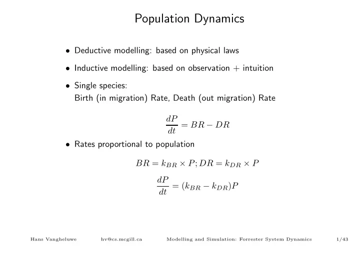
Population Dynamics • Deductive modelling: based on physical laws • Inductive modelling: based on observation + intuition • Single species: Birth (in migration) Rate, Death (out migration) Rate dP dt = BR − DR • Rates proportional to population BR = k BR × P ; DR = k DR × P dP dt = ( k BR − k DR ) P Hans Vangheluwe hv@cs.mcgill.ca Modelling and Simulation: Forrester System Dynamics 1/43
k BR = 1 . 4 , k DR = 1 . 2 : Exponential Growth trajectory population 2000000 1000000 0 10 20 30 40 50 Hans Vangheluwe hv@cs.mcgill.ca Modelling and Simulation: Forrester System Dynamics 2/43
k BR = 1 . 4 , k DR = 1 . 2 : log(Exponential Growth) trajectory 1E7 population 1E6 1E5 1E4 1E3 1E2 0 10 20 30 40 50 Hans Vangheluwe hv@cs.mcgill.ca Modelling and Simulation: Forrester System Dynamics 3/43
k BR = 1 . 2 , k DR = 1 . 4 : Exponential Decay trajectory 100 population 80 60 40 20 0 10 20 30 40 50 Hans Vangheluwe hv@cs.mcgill.ca Modelling and Simulation: Forrester System Dynamics 4/43
Logistic Model • Are k BR and k DR really constant ? • Energy consumption in a closed system → limits growth E pc = E tot P P ↑→ E pc ↓→ k BR ↓ and k DR ↑ until equilibrium • “crowding” effect: ecosystem can support maximum population P max dP P dt = k × (1 − ) × P P max • crowding is a quadratic effect Hans Vangheluwe hv@cs.mcgill.ca Modelling and Simulation: Forrester System Dynamics 5/43
k BR = 1 . 2 , k DR = 1 . 4 , crowding = 0 . 001 trajectory 200 population population 100 0 0 20 40 60 time Hans Vangheluwe hv@cs.mcgill.ca Modelling and Simulation: Forrester System Dynamics 6/43
Disadvantages • NO physical evidence for model structure ! • But, many phenomena can be well fitted by logistic model. • P max can only be estimated once steady-state has been reached. Not suitable for control, optimisation, . . . • Many-species system: P max , steady-state ? Hans Vangheluwe hv@cs.mcgill.ca Modelling and Simulation: Forrester System Dynamics 7/43
Multi-species: Predator-Prey • Individual species behaviour + interactions • Proportional to species, no interaction when one is extinct: product interaction P pred × P prey dP pred = − a × P pred + k × b × P pred × P prey dt dP prey = c × P prey − b × P pred × P prey dt • Excess death rate a > 0 , excess birth rate c > 0 , grazing factor b > 0 , efficiency factor 0 < k ≤ 1 • Lotka-Volterra equations (1956): periodic steady-state Hans Vangheluwe hv@cs.mcgill.ca Modelling and Simulation: Forrester System Dynamics 8/43
Predator Prey (population) trajectories predator prey 600 400 200 0 10 20 30 Hans Vangheluwe hv@cs.mcgill.ca Modelling and Simulation: Forrester System Dynamics 9/43
Predator Prey (phase) phaseplot predprey 300 200 100 200 400 600 Hans Vangheluwe hv@cs.mcgill.ca Modelling and Simulation: Forrester System Dynamics 10/43
Competition and Cooperation • Several species competing for the same food source dP 1 = a × P 1 − b × P 1 × P 2 dt dP 2 = c × P 2 − d × P 1 × P 2 dt • Cooperation of different species (symbiosis) dP 1 = − a × P 1 + b × P 1 × P 2 dt dP 2 = − c × P 2 + d × P 1 × P 2 dt Hans Vangheluwe hv@cs.mcgill.ca Modelling and Simulation: Forrester System Dynamics 11/43
Grouping and general n -species Interaction • Grouping (opposite of crowding) dP dt = − a × P + b × P 2 • n -species interaction n dP i � dt = ( a i + b ij × P j ) × P i , ∀ i ∈ { 1 , . . . , n } j =1 • Only binary interactions, no P 1 × P 2 × P 3 interactions Hans Vangheluwe hv@cs.mcgill.ca Modelling and Simulation: Forrester System Dynamics 12/43
Forrester System Dynamics • based on observation + physical insight • semi-physical, semi-inductive methodology Hans Vangheluwe hv@cs.mcgill.ca Modelling and Simulation: Forrester System Dynamics 13/43
Methodology 1. levels/stocks and rates/flows Level Inflow Outflow population birth rate death rate inventory shipments sales money income expenses 2. laundry list: levels, rates, and causal relationships birth rate → birth → population 3. Influence Diagram (+ and -) 4. Structure Diagram (functional relationships) dP dt = BR − DR Hans Vangheluwe hv@cs.mcgill.ca Modelling and Simulation: Forrester System Dynamics 14/43
Causal Relationships graduates standard of graduates SOL living (SOL) beer consumption time beer consumption latent variable SOL Hans Vangheluwe hv@cs.mcgill.ca Modelling and Simulation: Forrester System Dynamics 15/43
Archetypes • Bellinger http://www.outsights.com/systems/ • influence diagrams • Common combinations of reinforcing and balancing structures Hans Vangheluwe hv@cs.mcgill.ca Modelling and Simulation: Forrester System Dynamics 16/43
Archetypes: Reinforcing Loop state1 state2 Hans Vangheluwe hv@cs.mcgill.ca Modelling and Simulation: Forrester System Dynamics 17/43
Archetypes: Balancing Loop action state adjustment desired state Hans Vangheluwe hv@cs.mcgill.ca Modelling and Simulation: Forrester System Dynamics 18/43
Forrester System Dynamics uptake_predator loss_prey Grazing_efficiency prey_surplus_BR predator_surplus_DR Predator Prey 2−species predator−prey system Hans Vangheluwe hv@cs.mcgill.ca Modelling and Simulation: Forrester System Dynamics 19/43
Inductive Modelling: World Dynamics • BR : BirthRate • P : Population • POL : Pollution • MSL : Mean Standard of Living • . . . Hans Vangheluwe hv@cs.mcgill.ca Modelling and Simulation: Forrester System Dynamics 20/43
Inductive Modelling: Structure Characterization BR = f ( P, POL, MSL, . . . ) BR = BRN × f (1) ( P, POL, MSL, . . . ) BR = BRN × P × f (2) ( POL, MSL, . . . ) BR = BRN × P × f (3) ( POL ) × f (4) ( MSL ) . . . • f (3) ( POL ) inversely proportional • f (4) ( MSL ) proportional • compartmentalize to find correllations • . . . Structure Characterization ! Hans Vangheluwe hv@cs.mcgill.ca Modelling and Simulation: Forrester System Dynamics 21/43
Structure Characterisation: LSQ fit X 2 X(t) = - gt /2 + v_0 t X(t) = A sin (b t ) t 2 LSQ (sin) < LSQ (t ) Hans Vangheluwe hv@cs.mcgill.ca Modelling and Simulation: Forrester System Dynamics 22/43
Feature Extraction 1. Measurement data and model candidates 2. Structure selection and validation 3. Parameter estimation 4. Model use Hans Vangheluwe hv@cs.mcgill.ca Modelling and Simulation: Forrester System Dynamics 23/43
Feature Rationale Minimum Sensitivity to Noise Maximum Discriminating Power Hans Vangheluwe hv@cs.mcgill.ca Modelling and Simulation: Forrester System Dynamics 24/43
Throwing Stones Candidate Models 2 gt 2 + v 0 t 1. x = − 1 2. x = Asin ( bt ) Hans Vangheluwe hv@cs.mcgill.ca Modelling and Simulation: Forrester System Dynamics 25/43
Feature 1 (quadratic model) g i = 2 x i − 2 ˙ x i , i = A, B t 2 t i i F 1 = g A /g B Hans Vangheluwe hv@cs.mcgill.ca Modelling and Simulation: Forrester System Dynamics 26/43
Feature 2 (sin model) 1 b tg ( bt ) = x i x i ˙ solve numerically for b F 2 = 200 | b A − b B | b A + b B Hans Vangheluwe hv@cs.mcgill.ca Modelling and Simulation: Forrester System Dynamics 27/43
Feature Space Classification F2 = 200 |bA -bB|/(bA + bB) feature sin 1/b(tg(bt)) = xi/xi_der 2 Feature t F1 = gA/gB gi = 2xi/ti^2 - 2xi_der/ti Hans Vangheluwe hv@cs.mcgill.ca Modelling and Simulation: Forrester System Dynamics 28/43
Forrester’s World Dynamics model • “Club of Rome” World Dynamics model • Few “levels”, note the depletion of natural resources • implemented in Vensim PLE (www.vensim.com) Hans Vangheluwe hv@cs.mcgill.ca Modelling and Simulation: Forrester System Dynamics 29/43
Population & Food births material deaths pollution mult tab mult tab birth rate normal death rate normal birth rate normal 1 death rate normal 1 <pollution ratio> <material switch time 1 standard of switch time 3 living> <Time> <Time> Population births deaths births material multiplier deaths pollution multiplier births pollution multiplier deaths material multiplier population initial births births food multiplier deaths pollution deaths food multiplier crowding mult tab crowding births crowding multiplier multiplier deaths births food material land area <food mult tab births mult tab deaths population crowding crowding crowding density normal <material standard of mult tab> deaths food mult tab mult tab <pollution ratio> mult tab living> food crowding multiplier capital agriculture fraction indicated tab food ratio food pollution multiplier food capital agriculture fraction indicated <Time> pollution food per capita potential mult tab switch time 7 <capital ratio agriculture> food per food coefficient food per capita capita normal potential tab food coefficient 1 Hans Vangheluwe hv@cs.mcgill.ca Modelling and Simulation: Forrester System Dynamics 30/43
Recommend
More recommend
Explore More Topics
Stay informed with curated content and fresh updates.
