Polynomial preserving processes and discrete-tenor interest rate - PowerPoint PPT Presentation

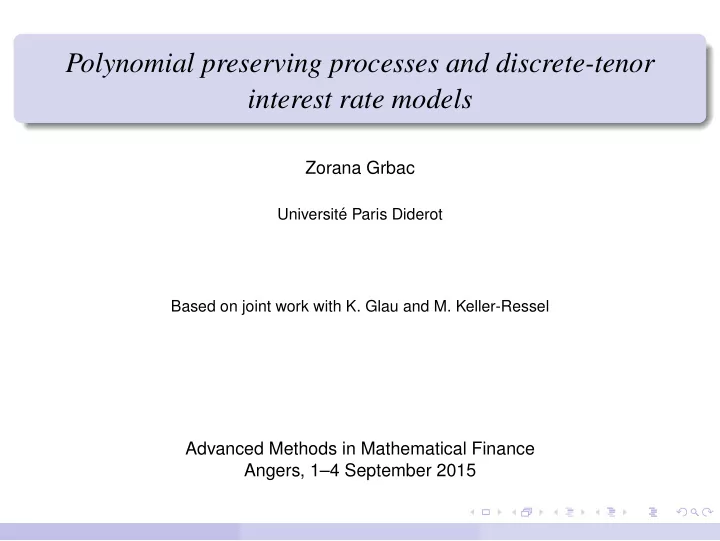
Polynomial preserving processes and discrete-tenor interest rate models Zorana Grbac Universit´ e Paris Diderot Based on joint work with K. Glau and M. Keller-Ressel Advanced Methods in Mathematical Finance Angers, 1–4 September 2015

Introduction and motivation Developing interest rate models that ensure on the one side nonnegative interest rates and/or spreads, and on the other side analytical pricing of both caplets and swaptions and enough flexibility for calibration, is a challenging problem. Recall: Caplet with strike K and maturity T k , settled in arrears: t = B ( t , T k + 1 ) δ k E P Tk + 1 [( L ( T k , T k ) − K ) + |F t ] Cpl k Swaption with swap rate S and exercise date T k – option to enter an interest rate swap: �� � + � � n n � � � Swp t = B ( t , T k ) E P Tk δ i L ( T k , T i ) B ( T k , T i ) − δ i SB ( T k , T i ) � F t i = k + 1 i = k + 1 �� � + � � n � � = B ( t , T k ) E P Tk 1 − c i B ( T k , T i ) � F t , i = k + 1 where c i = δ i S , for k + 1 ≤ i < n and c n = 1 + δ n S .

Interest rate models based on polynomial preserving processes Polynomial preserving processes seem to be very suitable to tackle these issues... Seminal paper introducing rational interest rate models: B. Flesaker and L.P . Hughston (1996). Positive interest Some references from recent literature: S. Cheng and M. Tehranchi (2014). Polynomial models for interest rates and stochastic volatility D. Filipovi´ c, M. Larsson and A. Trolle (2014). Linear-rational term structure models S. Cr´ epey, A. Macrina, T.M. Nguyen and D. Skovmand (2014). Rational multi-curve models with counterparty-risk valuation adjustments

Interest rate models based on polynomial preserving processes Polynomial preserving processes seem to be very suitable to tackle these issues... Seminal paper introducing rational interest rate models: B. Flesaker and L.P . Hughston (1996). Positive interest Some references from recent literature: S. Cheng and M. Tehranchi (2014). Polynomial models for interest rates and stochastic volatility D. Filipovi´ c, M. Larsson and A. Trolle (2014). Linear-rational term structure models S. Cr´ epey, A. Macrina, T.M. Nguyen and D. Skovmand (2014). Rational multi-curve models with counterparty-risk valuation adjustments In this paper: we work in the discrete-tenor setup and make use of the polynomial property already in the model construction to ensure the main theoretical and practical modeling requirements → we shall limit the presentation for simplicity to a single curve only

Introduction - main ingredients Discrete tenor structure: 0 = T 0 < T 1 < . . . < T n = T ∗ , with δ k = T k + 1 − T k , for all k T n = T ∗ T 0 T 1 T 2 t T k T k + 1 T n − 1 zero coupon bond with maturity T k : B ( t , T k ) B ( t , T k ) forward price process: F ( t , T k , T k + 1 ) = B ( t , T k + 1 ) forward Libor rate for the interval [ T k , T k + 1 ] : L ( t , T k ) Master relation 1 + δ k L ( t , T k ) = F ( t , T k , T k + 1 )

Forward measures forward martingale measure with numeraire B ( · , T k ) : P T k Density process for the change between two forward measures � d P T k = B ( 0 , T k + 1 ) B ( t , T k + 1 ) = F ( t , T k , T k + 1 ) B ( t , T k ) � � d P T k + 1 B ( 0 , T k ) F ( 0 , T k , T k + 1 ) F t No arbitrage: B ( · , T j ) B ( · , T k − 1 ) B ( · , T k ) ∈ M ( P T k ) , ∀ j , k ⇔ ∈ M ( P T k ) , ∀ k B ( · , T k ) Martingale condition F ( · , T k − 1 , T k ) , L ( · , T k − 1 ) ∈ M ( P T k ) .

Main modeling requirements Libor rates should be non-negative: L ( t , T k ) ≥ 0, for all t , k 1 The model should be arbitrage-free: L ( · , T k ) are P T k + 1 -martingales 2 The model should be analytically tractable: closed or semi-closed formulas for 3 most liquid derivatives (caps and swaptions) or efficient and accurate approximations The model should be flexible, i.e. provide good calibration 4 Post-crisis modeling: Libor rates depend on the tenor and also differ from the discounting rates = ⇒ various other rates have to be modeled in addition to (1), or equivalently their spreads = ⇒ the rates can become negative, whereas the spreads still always remain positive in the current market situation

New interest rate models – multiple curve setup Euribor - Eoniaswap spreads 250 spread 1m spread 3m spread 6m 200 spread 12m 150 bp 100 50 0 2006 2007 2008 2009 2010

Modeling of the forward price processes The forward price process with respect to the terminal tenor date: F ( t , T k , T n ) := B ( t , T k ) t ∈ [ 0 , T k ] , B ( t , T n ) , for all 1 ≤ k ≤ n . The modeling requirements now become: For all k = 1 , . . . , n − 1 and all t ∈ [ 0 , T k ] 1 1 ≤ F ( t , T k + 1 , T n ) ≤ F ( t , T k , T n ) The forward prices F ( · , T k , T n ) should be P T n -martingales 2 Tractability 3 Calibration (flexibility) 4

Comparison of some existing approaches Libor market model and extensions (Sandmann et al., Brace et al., Musiela and Rutkowski, Jamshidian, Eberlein and ¨ Ozkan, Joshi, Andersen et al., Rebonato, Schoenmakers et al.) L ( t , T k ) = L ( 0 , T k ) exp X k t , where X k are semimartingales Forward price models (Musiela and Rutkowski, Eberlein et al.) F ( t , T k , T k + 1 ) = F ( 0 , T k , T k + 1 ) exp X k t , where X k are semimartingales Affine Libor model (Keller-Ressel et al., Da Fonseca et al.) F ( t , T k , T n ) = E P Tn [ e � u k , X Tn � |F t ] = e φ Tn − t ( u k )+ � ψ Tn − t ( u k ) , X t � where X is an affine process

Additive construction of forward price models Instead of modeling directly the forward prices, we model the forward price spreads: S ( t , T k , T n ) := F ( t , T k , T n ) − F ( t , T k + 1 , T n ) for all k = 1 , . . . , n − 1. Then, requirements (1) and (2) become The forward price spreads S ( · , T k , T n ) are P T n -martingales and ( S ) S ( t , T k , T n ) ≥ 0 for all k = 1 , . . . , n and all t ∈ [ 0 , T k ] . The forward prices are sums of the forward price spreads: n � F ( t , T k , T n ) = S ( t , T j , T n ) j = k with � B ( t , T j ) − B ( t , T j + 1 ) for j < n , S ( t , T j , T n ) = B ( t , T n ) 1 for j = n .

Additive construction of forward price models Expressed in terms of bond prices, we have the following decomposition: B ( t , T k ) B ( t , T n ) = B ( t , T k ) − B ( t , T k + 1 ) + · · · + B ( t , T n − 1 ) − B ( t , T n ) + 1 B ( t , T n ) B ( t , T n ) � �� � � �� � ≥ 0 ≥ 0 and each summand is a P T n -martingale.

Additive construction of forward price models To specify the model, we set S ( t , T j , T n ) := S ( 0 , T j , T n ) N j t where the initial values S ( 0 , T j , T n ) are market data and ( N j ) 1 ≤ j ≤ n − 1 nonnegative P T n -martingales starting at 1. Furthermore, set E P Tn [ f j ( Y j T n ) |F t ] N j t := , E P Tn [ f j ( Y j T n )] where f j are nonnegative functions and Y j are semimartingales such that the conditional expectation above is analytically tractable. Our choice: polynomial functions and polynomial preserving processes

Caplets and swaptions – 2 Proposition The price of the caplet at time t ≤ T k is given by n �� � + � � � Cpl k µ j N j � F t t = B ( t , T n ) E P Tn T k j = k where µ k := S ( 0 , T k , T n ) and µ j := − δ k KS ( 0 , T j , T n ) , for j > k. Proposition The price of the swaption at time t ≤ T k is given by �� � + � � n � η j N j � F t Swp t = B ( t , T n ) E P Tn , T k j = k where η k := S ( 0 , T k , T n ) and η j := ( 1 − � j i = k + 1 c i ) S ( 0 , T j , T n ) , for j > k.

Polynomial preserving processes Let X be a time-homogeneous Markov process and a semimartingale on the state space E ⊂ R d , relative to some filtration ( F t ) t ≥ 0 Transition semigroup � P t f ( x ) := f ( y ) p t ( x , d y ) , E where ( p t ) t ≥ 0 is the transition kernel of X . Then E x [ f ( X t + s ) |F s ] = E X s [ f ( X t )] = P t f ( X s ) Denote by P m the vector space of polynomials on E up to degree m ≥ 0:   m   � α k x k , x ∈ E , α k ∈ R P m =  x �→  | k | = 0

Polynomial preserving processes Cuchiero, Keller-Ressel and Teichmann (2012), Filipovi´ c, Gourier, Mancini, Trolle (2012, 2013) The process X is m -polynomial preserving ( m -PP) if for all k ≤ m , P t ( P k ) ⊂ P k . Or equivalently: the generator A of X is m -polynomial preserving: A ( P k ) ⊂ P k , for all k ≤ m . for every k ≤ m , there exists a linear map A on P k such that � P k = e tA P t � If B = { e 1 , . . . , e M } denotes a basis of P k , then A = ( A ij ) i , j = 1 ,..., M is obtained from A e i = � M j = 1 A ij e j and P t f = ( α 1 , . . . , α M ) e tA ( e 1 , . . . , e M ) ⊤ , for any f = � M i = 1 α i e i ∈ P k

Polynomial preserving processes Hence: the expected value of any polynomial of ( X t ) is again a polynomial in the initial value X 0 = x Moments of X t can be computed explicitly and easily without knowing the probability distribution or characteristic function of X t : E x [( X t ) k ] = ( 0 , . . . , 0 , 1 , 0 , . . . , 0 ) e tA ( x 0 , x 1 , . . . , x m ) ⊤ , where we assumed d = 1 for simplicity. The only task is to compute the matrix exponential e tA