Polling Networks terminals terminals low-speedlines Terminal - - PDF document

polling networks
SMART_READER_LITE
LIVE PREVIEW

Polling Networks terminals terminals low-speedlines Terminal - - PDF document

Chapter 1 Polling Networks terminals terminals low-speedlines Terminal Personal Terminal Interchange Computer Interchange monitorlinks Central Computer Fullduplex high-speed connection Each station on the network is polled


slide-1
SLIDE 1

Chapter 1

Polling Networks

Central Computer Terminal Interchange Personal Computer Terminal Interchange

terminals low-speedlines terminals Fullduplex high-speed connection

monitorlinks

Each station on the network is polled in some predetermined order. When polled, a station uses the full data rate of the connecting channel to trans- mit its backlog of packets to the central computer. Between polls, stations accumulate messages in their queues, but do not transmit until they are polled. Transmissions between stations take place through the central computer, which receives all incoming packets and transmits them to the appropriate locations.

slide-2
SLIDE 2

EE414 Notes - Polling Mechanisms 2

BitSync Character Sync. Go-ahead Station Address Check Charaters Endof Packet Go-ahead Next Station BitSync Character Sync. Terminal Address Station Address Check Charaters Endof Packet Information Content (a)Pollingpacketforroll-callpolling (b)Formatfordatapackets (c)Suffixtolastdatapackettransmitted

Figure 1.1: Typical Packet Formats for Polling Network

1.1 Polling Mechanisms

Roll-Call Polling Each station has to be polled in turn by the central computer (controller). After the station has transmitted its backlog of messages, it notifies the central controller with a suffix to its last packet. After receiving this suffix packet, the controller sends a poll to the next station in the polling sequence. Hub Polling In this case the go-ahead (suffix) packet contains the next station address. A monitoring channel must be provided to indicate to the appropriate station that it should start transmitting. Essentially the go-ahead is transmitted directly from one station to another.

1.2 Roll-Call Polling Operation

Station

  • The central computer sends out a polling packet to station i in the

polling sequence.

slide-3
SLIDE 3

EE414 Notes - Roll-Call Polling Operation 3

  • Station i synchronises on bits and characters.
  • Station i reads and interprets the station address and the go-ahead

contained in the polling packet.

  • Station i transmits all its backlogged messages to the central computer

for distribution to the central computer and other stations.

  • Station i appends a go-ahead, and possibly a next-station address to

its last packet. Controller

  • The central computer synchronises on bits and characters.
  • The central computer reads and interprets the incoming packets, in-

cluding the final go-ahead and next station address.

  • The central computer sends out a poll to station (i + 1).

These steps are repeated for each station. When all stations have been polled the whole sequence begins again. The communications between the controller and stations may be half-duplex

  • r duplex. We assume duplex.

Transmission from Controller to Stations: This can be asynchronous

  • r continuous. If continuous then step 2 of station operation can be ignored.

Transmission from Station to Controller: This is asynchronous. If a station has no messages it either does not reply or sends back a go-ahead packet.

slide-4
SLIDE 4

EE414 Notes - Polling Analysis Model 4

1.3 Polling Analysis Model

Controller Station1 Station i Station2 Station M

Direction

  • fPoll

Figure 1.2: A Typical Polling Network Messages arrive at random at each station and are stored in a buffer until the station is polled. When polled, the station transmits all packets in its buffer and finishes by sending a go-ahead packet. The next station is then polled on a roll-call or hub basis. A walk time (w) is required to transfer the poll from one station to another.

1.3.1 Model Assumptions

In determining the performance, the following assumptions are made:

  • Each station has the same Poisson arrival statistics with average arrival

rate λ packets/second.

  • The walk time (w) between stations is constant and the same for every

consecutive station.

slide-5
SLIDE 5

EE414 Notes - Polling Analysis Model 5

  • The channel propagation times between stations are equal and are

included in the walk time.

  • Packet length distributions are the same for packets arriving at each

station.

1.3.2 Average Cycle Time

Let: Nm = Average number of packets stored at a station when poll arrives ¯ X = Average length of packet (in bits) R = Speed of transmission channel (in bits per second) Nm ¯ X/R = Time needed to empty station buffer (in seconds) The next stations starts transmitting after the walk time w. Length of average cycle time = Tc = M[Nm ¯ X/R + w] where M is the number of stations. From the input statistics: Nm = λTc Combining this with the previous equation to eliminate Nm gives: Tc = Mw 1 − Mλ ¯ X/R Define throughput S = Mλ ¯ X/R Therefore: Tc = Mw 1 − S seconds S must be < 1 in order to have finite buffer lengths at stations.

slide-6
SLIDE 6

EE414 Notes - Polling Analysis Model 6

1.3.3 Delay Analysis

Let W = average time an arriving packet must wait before reaching the head of the queue. This delay is made up of two components:

  • 1. The waiting delay (W1) in the station buffer while other stations are

being served,

  • 2. The waiting delay (W2) in the station buffer while that particular

station is being served. W = W1 + W2

Service Station i Service Station i Packet Arrival Packet Departure W1 W W2 Time

Figure 1.3: Division of Waiting Times for a Typical Packet For W1 The average number of packets that are transmitted over channel from sta- tion = λTc. Average service time = λTc ¯ X R Define ρ = λ ¯ X R = S M Service time per station = ρTc Remaining part of average cycle during which the station is idle is: Tc(1 − ρ) Random arrivals occur in the interval Tc(1 − ρ)

slide-7
SLIDE 7

EE414 Notes - Polling Analysis Model 7 On average the delay is: Tc(1 − ρ) 2 seconds Using the previous expression for Tc: W1 = Mw(1 − ρ) 2(1 − Mρ)

Service Station i+1 (1- )Tc

ñ ñTc

w Service Station i Service Station1 w Service Station M Service Station i Tc

Figure 1.4: A Cycle for a Polling Network, with Average Time Indicated For W2 An approximation is used. Consider an equivalent network for which there is no walk time so that there is always some station being served if there are packets in the network. Think of the whole system as having input Mλ and only a single server. An M/G/1 model will apply. The delay in a buffer for an M/G/1 system is: W ′ = λ′ 2(1 − ρ′)E[τ 2] where E[τ 2] = σ2 + 1/µ2 is the 2nd moment of the service time distribution. In our case λ′ = Mλ ρ′ = Mρ = S E[τ 2] = X R 2 = X2 R2

slide-8
SLIDE 8

EE414 Notes - Polling Analysis Model 8 Therefore W2 = Mλ(X2/R2) 2(1 − S) = Mλ ¯ X R 1 2(1 − S) 1 ¯ XR X2 As S = Mλ ¯ X/R W2 = SX2 2 ¯ XR(1 − S) Total delay is W1 + W2 so W = Mw(1 − ρ) 2(1 − Mρ) + SX2 2 ¯ XR(1 − S) Rewriting, the average time a packet must wait before reaching the head of the queue in a polling network is: W = Mw(1 − S/M) 2(1 − S) + SX2 2 ¯ XR(1 − S) Two distributions of packet lengths are of interest: Constant: X2 = ( ¯ X)2 W = Mw(1 − S/M) 2(1 − S) + S ¯ X 2R(1 − S) Exponential: X2 = 2( ¯ X)2 W = Mw(1 − S/M) 2(1 − S) + S ¯ X R(1 − S)

slide-9
SLIDE 9

EE414 Notes - Polling Network Example 9

1.4 Polling Network Example

Consider a metropolitan area network with a single central processor located at the headend of a broadband CATV system that has a tree topology. The following are specified:

  • Maximum distance from headend to a subscriber station - 20 km
  • Access technique - roll-call poling
  • Length of polling packet - 8 bytes
  • Length of go-ahead - 1 byte
  • Data rate of channel - 56 kbps
  • Number of subscribers - 1000
  • Packet length distribution (subscriber to headend) - exponential
  • Mean packet length - 200 bytes
  • Propagation delay - 6 µs/km
  • Mode of transmission - duplex
  • Modem synchronisation time (at headend) - 10 ms

(a) Find the mean waiting time (delay) for arriving packets at the stations if each user generates an average of one packet per minute. (b) If the channel data rate is reduced to 9,600 bps, what is the largest possible mean packet length that will not overload the system. (c) For mean packet lengths of 2/3 the result found for (b), determine the mean waiting delay. First determine walk time (w). This is made up of:

  • Tx time for go-ahead
  • Propagation delay of go-ahead
slide-10
SLIDE 10

EE414 Notes - Polling Network Example 10

  • Tx delay for polling packet
  • Propagation delay for polling packet
  • Sync. delay of modem for received data at headend

Calculating these:

  • 8/(56 × 103) = 0.14 ms
  • 20 × 6 = 120µs = 0.12 ms
  • 8 × 8/(56 × 103) = 1.14 ms
  • 0.12 ms
  • 10 ms

Total = 11.52 ms. (a) Throughput per station = ρ = λ ¯ X R = 1/60 × 200 × 8 56 × 103 = 4.76 × 10⁻⁴ Total throughput = S = Mρ = 1000 × 4.76 × 10−4 = 0.476 Mean Delay = W = Mw(1 − S/M) 2(1 − S) + S ¯ X R(1 − S) W = 1000(11.52 × 10⁻³)(1 − 4.76 × 10⁻⁴) 2(1 − 0.476) + 0.476 × 200 × 8 56 × 103(1 − 0.476) = 10.99 + 0.026 = 11.02 sec (b) SMAX = 1000(1/60 × 8 × ¯ XMAX) 9600 < 1 ¯ XMAX < 72 bytes

slide-11
SLIDE 11

EE414 Notes - Polling Network Example 11 (c) ¯ X = 2/3 × 72 = 48 bytes throughput per station = ρ = λ ¯ X R = 1/60 × 48 × 8 9600 = 6.67 × 10⁻⁴ total throughput = S = Mρ = 1000 × 6.67 × 10−4 = 0.67 Polling packet and go-ahead transmission times change because of the new channel bit rate. New walk time is given by: w = 8 × 8 9.6 + 8 9.6 + 2 × 0.12 + 10 = 17.74 ms Therefore W is given by: W = 26.62 + 0.01 = 26.63 sec Note that W in both cases is dominated by W1 (W2 ≈ 0).

slide-12
SLIDE 12

Chapter 2

Ring Networks

station ring interface unit

Figure 2.1: A Typical Ring Structure A ring network is characterised by a sequence of point-to-point links between stations, forming a loop. All messages travel in one direction around the loop, passing through network interfaces at each station.

2.1 Operation of Ring

Bits from the ring enter in one direction in a serial fashion and, after a delay

  • f several bits, are retransmitted over the ring either unchanged, or after

some modification.

slide-13
SLIDE 13

EE414 Notes - Operation of Ring 13 Access to the ring for transmissions in controlled by a token. A station wishing to transmit waits for an idle token to arrive. It then changes it into a busy token and follows it with data. An idle token is transmitted at the end of the holding time. In the listen mode, each station passes on the packet received at its input after a delay referred to as the station latency. Define: Ring Latency = Station Latency + Propagation Delay The operational mode of a ring is determined by when idle tokens may be

  • generated. The modes are:
  • Multiple-Token
  • Single-Token
  • Single-Packet
slide-14
SLIDE 14

EE414 Notes - Operation of Ring 14

LineDriver Controller LineReceiver Receiver Transmitter TransmitBuffer ReceiveBuffer AttachedDevice Delay

Ring Input Ring Output Node in Node

  • ut

Node in Node

  • ut

ListenMode

Ring Input Ring Output

Delay

Node in Node

  • ut

TransmitMode

Ring Input Ring Output

Figure 2.2: Station / Ring Interface

slide-15
SLIDE 15

EE414 Notes - Operation of Ring 15 Figure 2.3: Operational Modes of Ring

slide-16
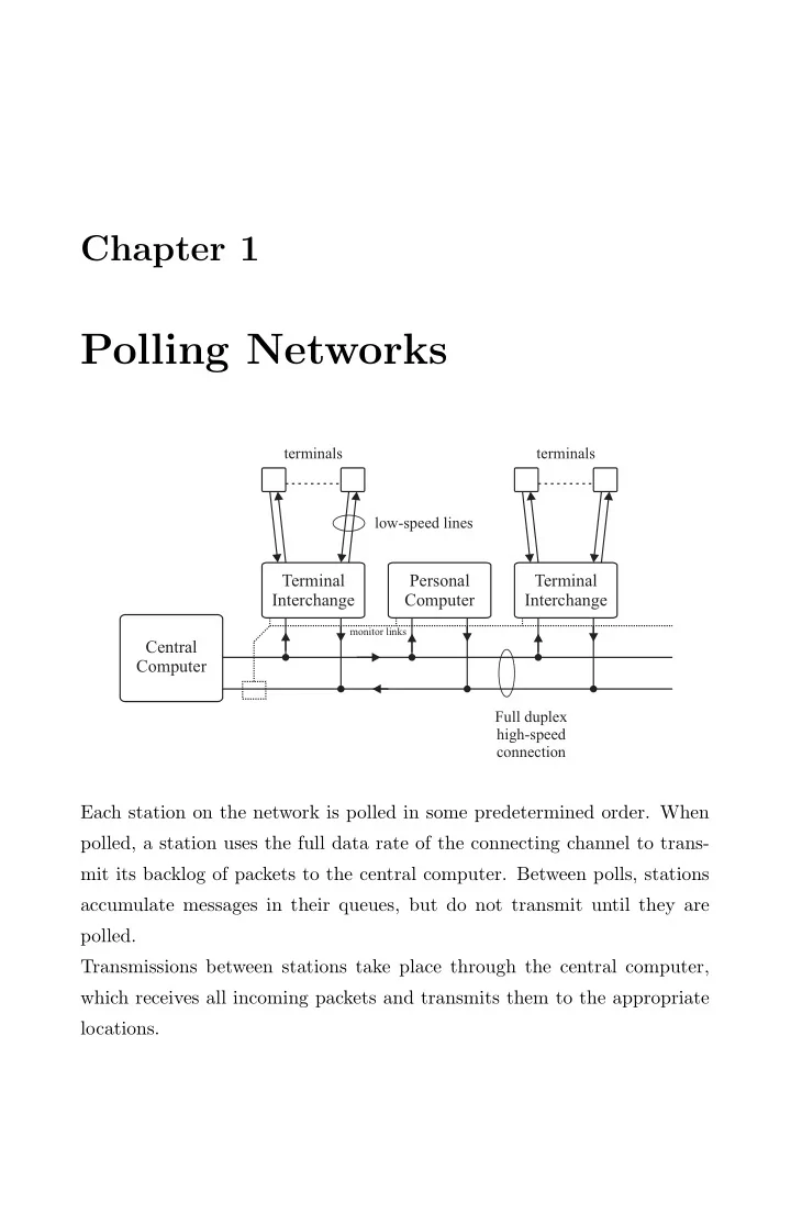
SLIDE 16

EE414 Notes - Delay Analysis for Token Ring Networks 16

2.2 Delay Analysis for Token Ring Networks

The following assumptions are made in the analysis:

  • All stations behave the same.
  • The arrival process at each station is Poisson with average arrival rate
  • f λ.
  • The average distance between the sending and receiving station is 1

2

the distance around the ring.

  • The stations are spaced so that the propagation delays between con-

secutively serviced stations are equal and given by τ/M, where τ is the total ring propagation delay and M is the number of stations.

  • The packet length distribution is the same for each station with mean

length ¯ X bits and second moment X2.

  • All packets queued at a station are transmitted during a service period.

Let: R = Channel bit rate (bits/sec) B = Latency per station (bits) τ = Round trip propagation delay for the ring (sec) τ ′ = Ring Latency (sec) A common channel is used for both a token ring network and a polling

  • network. The master controller is not of importance to the operation of the

system in so far as the analysis is concerned. Thus, the polling equations, developed in the previous chapter, can be used for token ring analysis. The average waiting time in a polling network was derived to be: W = Mw(1 − S/M) 2(1 − S) + S(X/R)2 2( ¯ X/R)(1 − S) The average transfer delay T is given by T = ¯ X/R + τavg + W

slide-17
SLIDE 17

EE414 Notes - Delay Analysis for Token Ring Networks 17 where ¯ X/R = Average time to transmit a packet τavg = Average latency from Tx station to Rx station We need to state what τavg is for a token ring LAN. We assume that a packet travels on average half way around the ring before it reaches its destination station. τ ′ = τ + MB/R and τavg = τ ′/2. The expression for W must be determined for token ring operation. Need to evaluate:

  • 1. The walk time (w)
  • 2. Moments of the service time ¯

X/R and X2/R2

  • 3. The network throughput
  • 1. Walk Time

w = τ ′/M = B/R + τ/M

  • 2. Service Time

For ring networks, the service time can include any time interval during which the ring is inactive in the course of completing one packet transmis- sion and becoming available for another transmission. Call this time the Effective Service Time E.

  • 3. Network Throughput

define S′ = Mλ ¯ E while S = Mλ ¯ X/R

slide-18
SLIDE 18

EE414 Notes - Delay Analysis for Token Ring Networks 18 Using these expressions gives T = ¯ X R + τ ′ 2 + τ ′(1 − S′/M) 2(1 − S′) + S′E2 2 ¯ E(1 − S′) This gives a general expression for the delay in a token ring network. The expressions for ¯ E, E2 and S′ will depend on the operational mode of the ring and the packet length distribution. Note that T is normally referred to as the unnormalised delay. The nor- malised delay is defined as: ˆ T = T ( ¯ X/R)

slide-19
SLIDE 19

EE414 Notes - Multiple Token Operation 19

2.3 Multiple Token Operation

In this case a new token is generated immediately after the last bit of the packet leaves the transmitting station. This is similar to the polling case as the ring is always transmitting between walk times. The average effective service time is ¯ X/R and the second moment is X2/R2. Average transfer delay is therefore: T = ¯ X R + τ ′ 2 + τ ′(1 − S/M) 2(1 − S) + SX2 2 ¯ XR(1 − S) Maximum throughput is obtained when S = 1. However S = 1 ⇒ T → ∞ which is not desirable. For fixed length and exponentially distributed packet lengths we have: Fixed Length Packets [X2 = ( ¯ X)2] T = ¯ X R + τ ′ 2 + τ ′(1 − S/M) 2(1 − S) + S ¯ X/R 2(1 − S) Exponentially Distributed Packet Lenghts [X2 = 2( ¯ X)2] T = ¯ X R + τ ′ 2 + τ ′(1 − S/M) 2(1 − S) + S ¯ X/R (1 − S) Note: In practice, maximum throughput is determined as the largest through- put for which the average transfer delay remains finite.

2.4 Single Token Operation

A new free token is not generated until the busy token from that station has been received again, i.e. has circled the ring.

slide-20
SLIDE 20

EE414 Notes - Single Token Operation 20 Case 1 If the packet transmission time X/R is greater than the ring latency τ ′, the station is still transmitting a packet when its busy token returns after circulating around the ring. In this case the operation is the same as the multiple token case. Case 2 If X/R < τ ′, single token operation is different. In this case, the effective service time is > X/R due to periods in which the ring is waiting for the busy token to return. Define normalised ring latency delay: a′ = τ ′ ¯ X/R Fixed and exponentially distributed packets must be treated differently. Fixed Length Packets ¯ X = X = constant. If a′ < 1 then the multiple token result applies. If a′ > 1 then the result is different. In this case, the ring cannot be used to transmit another packet until the token has completed its ”tour” of the ring. ¯ E = τ ′ S′ = Mλτ ′ = Mλ( ¯ X/R)a′ = Sa′ Substituting into the general equation for T gives: T = ¯ X R + τ ′ 2 + τ ′(1 − Sa′/M) 2(1 − Sa′) + Sa′τ ′ 2(1 − Sa′) If a′ < 1 then the maximum achievable throughput on the ring is 1 If a′ > 1 the throughput can reach a maximum of 1/a′ (Noting that maximum throughput is found by setting S′ = 1 and finding the corresponding value of S.)

slide-21
SLIDE 21

EE414 Notes - Single Token Operation 21 Exponential Packet Distribution In this case the packet length is random. A probability distribution must be assigned to the effective service time. If X/R < τ ′ then E = τ ′ If X/R > τ ′ then E = X/R X has an exponential distribution function with mean ¯ X and since R is a constant, the distribution function of X/R is: FX/R(y) =

  • 1 − e−Ry/ ¯

X,

y ≥ 0 0 , y < 0 So the distribution function of the effective service time is: FE(y) =

  • 0 ,

y < τ ′ 1 − e−Ry/ ¯

X,

y ≥ τ ′

ô' X/R F (y)

X/R

1 y ô' X/R y 1 F (y)

E

slide-22
SLIDE 22

EE414 Notes - Single Token Operation 22 The first and second moments of E are: ¯ E = ( ¯ X/R)e−a′ + τ ′ E2 = (τ ′)2 + 2( ¯ X/R)2e−a′(1 + a′) And also S′ = Se−a′ + Sa′ thus: T = ¯ X R + τ ′ 2 + τ ′[1 − S(e−a′ + a′)/M] 2[1 − S(e−a′ + a′)] + ¯ X R S[(a′)2 + 2(1 + a′)e−a′] 2[1 − S(e−a′ + a′)] The maximum throughput obtainable is given by 1 e−a′ + a′

slide-23
SLIDE 23

EE414 Notes - Single Packet Operation 23

2.5 Single Packet Operation

In this mode of operation there is never more than one packet circulating

  • n the ring.

There is always a delay of τ ′ seconds after the end of each packet. Therefore: E = X/R + τ ′ The 1st and 2nd moments are: ¯ E = ¯ X/R + τ ′ E2 = (X/R)2 + 2τ ′( ¯ X/R) + (τ ′)2 This results in the average delay expression: T = ¯ X R + τ ′ 2 + τ ′[1 − (1 + a′)S/M] 2[1 − (1 + a′)S] + S[X2 + (Rτ ′)2 + 2 ¯ XRτ ′] 2[1 − (1 + a′)S]R ¯ X] Fixed Length Packets T = ¯ X R + τ ′ 2 + τ ′[1 − (1 + a′)S/M] 2[1 − (1 + a′)S] + S( ¯ X/R)(1 + a′)2 2[1 − (1 + a′)S] Exponentially Distributed Packet Lengths T = ¯ X R + τ ′ 2 + τ ′[1 − (1 + a′)S/M] 2[1 − (1 + a′)S] + S( ¯ X/R)[(1 + a′)2 + 1] 2[1 − (1 + a′)S] Upper bound to throughput is 1/(1 + a′)