Plan of the Lecture Review: state-space notions: canonical forms, - - PowerPoint PPT Presentation

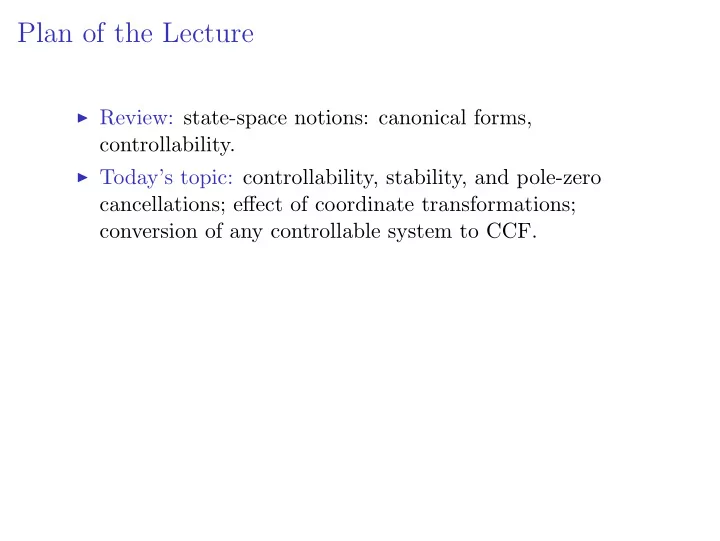
Plan of the Lecture

◮ Review: state-space notions: canonical forms,

controllability.

◮ Today’s topic: controllability, stability, and pole-zero

cancellations; effect of coordinate transformations; conversion of any controllable system to CCF.

Plan of the Lecture

◮ Review: state-space notions: canonical forms,

controllability.

◮ Today’s topic: controllability, stability, and pole-zero

cancellations; effect of coordinate transformations; conversion of any controllable system to CCF. Goal: explore the effect of pole-zero cancellations on internal stability; understand the effect of coordinate transformations on the properties of a given state-space model (transfer function;

• pen-loop poles; controllability).

Plan of the Lecture

◮ Review: state-space notions: canonical forms,

controllability.

◮ Today’s topic: controllability, stability, and pole-zero

cancellations; effect of coordinate transformations; conversion of any controllable system to CCF. Goal: explore the effect of pole-zero cancellations on internal stability; understand the effect of coordinate transformations on the properties of a given state-space model (transfer function;

• pen-loop poles; controllability).

Reading: FPE, Chapter 7

State-Space Realizations

˙ x = Ax + Bu y = Cx u y

State-Space Realizations

˙ x = Ax + Bu y = Cx u y

◮ a given transfer function G(s) can be realized using

infinitely many state-space models

State-Space Realizations

˙ x = Ax + Bu y = Cx u y

◮ a given transfer function G(s) can be realized using

infinitely many state-space models

◮ certain properties make some realizations preferable to

• thers

State-Space Realizations

˙ x = Ax + Bu y = Cx u y

◮ a given transfer function G(s) can be realized using

infinitely many state-space models

◮ certain properties make some realizations preferable to

• thers

◮ one such property is controllability

Controllability Matrix

Consider a single-input system (u ∈ R): ˙ x = Ax + Bu, y = Cx x ∈ Rn The Controllability Matrix is defined as C(A, B) =

• B | AB | A2B | . . . | An−1B
• We say that the above system is controllable if its

controllability matrix C(A, B) is invertible.

Controllability Matrix

Consider a single-input system (u ∈ R): ˙ x = Ax + Bu, y = Cx x ∈ Rn The Controllability Matrix is defined as C(A, B) =

• B | AB | A2B | . . . | An−1B
• We say that the above system is controllable if its

controllability matrix C(A, B) is invertible.

◮ As we will see later, if the system is controllable, then we

may assign arbitrary closed-loop poles by state feedback of the form u = −Kx.

Controllability Matrix

Consider a single-input system (u ∈ R): ˙ x = Ax + Bu, y = Cx x ∈ Rn The Controllability Matrix is defined as C(A, B) =

• B | AB | A2B | . . . | An−1B
• We say that the above system is controllable if its

controllability matrix C(A, B) is invertible.

◮ As we will see later, if the system is controllable, then we

may assign arbitrary closed-loop poles by state feedback of the form u = −Kx.

◮ Whether or not the system is controllable depends on its

state-space realization.

Example: Computing C(A, B)

Let’s get back to our old friend: ˙ x1 ˙ x2

• =

1 −6 −5

• A

x1 x2

• +

1

• B

u, y =

• 1

1

• C

x1 x2

Example: Computing C(A, B)

Let’s get back to our old friend: ˙ x1 ˙ x2

• =

1 −6 −5

• A

x1 x2

• +

1

• B

u, y =

• 1

1

• C

x1 x2

• Here, x ∈ R2 =

⇒ A ∈ R2×2 = ⇒ C(A, B) ∈ R2×2

Example: Computing C(A, B)

Let’s get back to our old friend: ˙ x1 ˙ x2

• =

1 −6 −5

• A

x1 x2

• +

1

• B

u, y =

• 1

1

• C

x1 x2

• Here, x ∈ R2 =

⇒ A ∈ R2×2 = ⇒ C(A, B) ∈ R2×2 C(A, B) = [B | AB]

Example: Computing C(A, B)

Let’s get back to our old friend: ˙ x1 ˙ x2

• =

1 −6 −5

• A

x1 x2

• +

1

• B

u, y =

• 1

1

• C

x1 x2

• Here, x ∈ R2 =

⇒ A ∈ R2×2 = ⇒ C(A, B) ∈ R2×2 C(A, B) = [B | AB] AB = 1 −6 −5 1

• =

1 −5

Example: Computing C(A, B)

Let’s get back to our old friend: ˙ x1 ˙ x2

• =

1 −6 −5

• A

x1 x2

• +

1

• B

u, y =

• 1

1

• C

x1 x2

• Here, x ∈ R2 =

⇒ A ∈ R2×2 = ⇒ C(A, B) ∈ R2×2 C(A, B) = [B | AB] AB = 1 −6 −5 1

• =

1 −5

• =

⇒ C(A, B) = 1 1 −5

Example: Computing C(A, B)

Let’s get back to our old friend: ˙ x1 ˙ x2

• =

1 −6 −5

• A

x1 x2

• +

1

• B

u, y =

• 1

1

• C

x1 x2

• Here, x ∈ R2 =

⇒ A ∈ R2×2 = ⇒ C(A, B) ∈ R2×2 C(A, B) = [B | AB] AB = 1 −6 −5 1

• =

1 −5

• =

⇒ C(A, B) = 1 1 −5

• Is this system controllable?

Example: Computing C(A, B)

Let’s get back to our old friend: ˙ x1 ˙ x2

• =

1 −6 −5

• A

x1 x2

• +

1

• B

u, y =

• 1

1

• C

x1 x2

• Here, x ∈ R2 =

⇒ A ∈ R2×2 = ⇒ C(A, B) ∈ R2×2 C(A, B) = [B | AB] AB = 1 −6 −5 1

• =

1 −5

• =

⇒ C(A, B) = 1 1 −5

• Is this system controllable?

det C = −1 = 0 = ⇒ system is controllable

Controller Canonical Form

A single-input state-space model ˙ x = Ax + Bu, y = Cx is said to be in Controller Canonical Form (CCF) is the matrices A, B are of the form A =        1 . . . 1 . . . . . . . . . . . . ... . . . . . . . . . 1 ∗ ∗ ∗ . . . ∗ ∗        , B =        . . . 1        A system in CCF is always controllable!!

(The proof of this for n > 2 uses the Jordan canonical form, we will not worry about this.)

CCF with Arbitrary Zeros

In our example, we had G(s) = s + 1 s2 + 5s + 6, with a minimum-phase zero at z = −1.

CCF with Arbitrary Zeros

In our example, we had G(s) = s + 1 s2 + 5s + 6, with a minimum-phase zero at z = −1. Let’s consider a general zero location s = z: G(s) = s − z s2 + 5s + 6

CCF with Arbitrary Zeros

In our example, we had G(s) = s + 1 s2 + 5s + 6, with a minimum-phase zero at z = −1. Let’s consider a general zero location s = z: G(s) = s − z s2 + 5s + 6 This gives us a CCF realization ˙ x1 ˙ x2

• =

1 −6 −5

• A

x1 x2

• +

1

• B

u, y =

• −z

1

• C

x1 x2

CCF with Arbitrary Zeros

In our example, we had G(s) = s + 1 s2 + 5s + 6, with a minimum-phase zero at z = −1. Let’s consider a general zero location s = z: G(s) = s − z s2 + 5s + 6 This gives us a CCF realization ˙ x1 ˙ x2

• =

1 −6 −5

• A

x1 x2

• +

1

• B

u, y =

• −z

1

• C

x1 x2

• Since A, B are the same, C(A, B) is the same =

⇒ the system is still controllable.

CCF with Arbitrary Zeros

In our example, we had G(s) = s + 1 s2 + 5s + 6, with a minimum-phase zero at z = −1. Let’s consider a general zero location s = z: G(s) = s − z s2 + 5s + 6 This gives us a CCF realization ˙ x1 ˙ x2

• =

1 −6 −5

• A

x1 x2

• +

1

• B

u, y =

• −z

1

• C

x1 x2

• Since A, B are the same, C(A, B) is the same =

⇒ the system is still controllable. A system in CCF is controllable for any locations of the zeros.

OCF with Arbitrary Zeros

Start with the CCF ˙ x1 ˙ x2

• =

1 −6 −5

• A

x1 x2

• +

1

• B

u, y =

• −z

1

• C

x1 x2

OCF with Arbitrary Zeros

Start with the CCF ˙ x1 ˙ x2

• =

1 −6 −5

• A

x1 x2

• +

1

• B

u, y =

• −z

1

• C

x1 x2

• Convert to OCF:

(A → AT , B → CT , C → BT ) ˙ x1 ˙ x2

• =

−6 1 −5

• ¯

A=AT

x1 x2

• +

−z 1

• ¯

B=CT

u, y =

• 1
• ¯

C=BT

x1 x2

OCF with Arbitrary Zeros

Start with the CCF ˙ x1 ˙ x2

• =

1 −6 −5

• A

x1 x2

• +

1

• B

u, y =

• −z

1

• C

x1 x2

• Convert to OCF:

(A → AT , B → CT , C → BT ) ˙ x1 ˙ x2

• =

−6 1 −5

• ¯

A=AT

x1 x2

• +

−z 1

• ¯

B=CT

u, y =

• 1
• ¯

C=BT

x1 x2

• We already know that this system realizes the same t.f. as the
• riginal system.

OCF with Arbitrary Zeros

Start with the CCF ˙ x1 ˙ x2

• =

1 −6 −5

• A

x1 x2

• +

1

• B

u, y =

• −z

1

• C

x1 x2

• Convert to OCF:

(A → AT , B → CT , C → BT ) ˙ x1 ˙ x2

• =

−6 1 −5

• ¯

A=AT

x1 x2

• +

−z 1

• ¯

B=CT

u, y =

• 1
• ¯

C=BT

x1 x2

• We already know that this system realizes the same t.f. as the
• riginal system.

But is it controllable?

OCF with Arbitrary Zeros

˙ x1 ˙ x2

• =

−6 1 −5

• ¯

A=AT

x1 x2

• +

−z 1

• ¯

B=CT

u, y =

• 1
• ¯

C=BT

x1 x2

OCF with Arbitrary Zeros

˙ x1 ˙ x2

• =

−6 1 −5

• ¯

A=AT

x1 x2

• +

−z 1

• ¯

B=CT

u, y =

• 1
• ¯

C=BT

x1 x2

• Let’s find the controllability matrix:

OCF with Arbitrary Zeros

˙ x1 ˙ x2

• =

−6 1 −5

• ¯

A=AT

x1 x2

• +

−z 1

• ¯

B=CT

u, y =

• 1
• ¯

C=BT

x1 x2

• Let’s find the controllability matrix:

C( ¯ A, ¯ B) = ¯ B | ¯ A ¯ B

OCF with Arbitrary Zeros

˙ x1 ˙ x2

• =

−6 1 −5

• ¯

A=AT

x1 x2

• +

−z 1

• ¯

B=CT

u, y =

• 1
• ¯

C=BT

x1 x2

• Let’s find the controllability matrix:

C( ¯ A, ¯ B) = ¯ B | ¯ A ¯ B

• ¯

A ¯ B = −6 1 −5 −z 1

OCF with Arbitrary Zeros

˙ x1 ˙ x2

• =

−6 1 −5

• ¯

A=AT

x1 x2

• +

−z 1

• ¯

B=CT

u, y =

• 1
• ¯

C=BT

x1 x2

• Let’s find the controllability matrix:

C( ¯ A, ¯ B) = ¯ B | ¯ A ¯ B

• ¯

A ¯ B = −6 1 −5 −z 1

• =
• −6

−z − 5

OCF with Arbitrary Zeros

˙ x1 ˙ x2

• =

−6 1 −5

• ¯

A=AT

x1 x2

• +

−z 1

• ¯

B=CT

u, y =

• 1
• ¯

C=BT

x1 x2

• Let’s find the controllability matrix:

C( ¯ A, ¯ B) = ¯ B | ¯ A ¯ B

• ¯

A ¯ B = −6 1 −5 −z 1

• =
• −6

−z − 5

• ∴ C( ¯

A, ¯ B) = −z −6 1 −z − 5

OCF with Arbitrary Zeros

˙ x1 ˙ x2

• =

−6 1 −5

• ¯

A=AT

x1 x2

• +

−z 1

• ¯

B=CT

u, y =

• 1
• ¯

C=BT

x1 x2

• Let’s find the controllability matrix:

C( ¯ A, ¯ B) = ¯ B | ¯ A ¯ B

• ¯

A ¯ B = −6 1 −5 −z 1

• =
• −6

−z − 5

• ∴ C( ¯

A, ¯ B) = −z −6 1 −z − 5

• det C = z(z + 5) + 6

OCF with Arbitrary Zeros

˙ x1 ˙ x2

• =

−6 1 −5

• ¯

A=AT

x1 x2

• +

−z 1

• ¯

B=CT

u, y =

• 1
• ¯

C=BT

x1 x2

• Let’s find the controllability matrix:

C( ¯ A, ¯ B) = ¯ B | ¯ A ¯ B

• ¯

A ¯ B = −6 1 −5 −z 1

• =
• −6

−z − 5

• ∴ C( ¯

A, ¯ B) = −z −6 1 −z − 5

• det C = z(z + 5) + 6 = z2 + 5z + 6

OCF with Arbitrary Zeros

˙ x1 ˙ x2

• =

−6 1 −5

• ¯

A=AT

x1 x2

• +

−z 1

• ¯

B=CT

u, y =

• 1
• ¯

C=BT

x1 x2

• Let’s find the controllability matrix:

C( ¯ A, ¯ B) = ¯ B | ¯ A ¯ B

• ¯

A ¯ B = −6 1 −5 −z 1

• =
• −6

−z − 5

• ∴ C( ¯

A, ¯ B) = −z −6 1 −z − 5

• det C = z(z + 5) + 6 = z2 + 5z + 6 = 0

for z = −2 or z = −3

OCF with Arbitrary Zeros

˙ x1 ˙ x2

• =

−6 1 −5

• ¯

A=AT

x1 x2

• +

−z 1

• ¯

B=CT

u, y =

• 1
• ¯

C=BT

x1 x2

• Let’s find the controllability matrix:

C( ¯ A, ¯ B) = ¯ B | ¯ A ¯ B

• ¯

A ¯ B = −6 1 −5 −z 1

• =
• −6

−z − 5

• ∴ C( ¯

A, ¯ B) = −z −6 1 −z − 5

• det C = z(z + 5) + 6 = z2 + 5z + 6 = 0

for z = −2 or z = −3 The OCF realization of the transfer function G(s) = s − z s2 + 5s + 6 is not controllable when z = −2 or −3, even though the CCF is always controllable.

Beware of Pole-Zero Cancellations!

The OCF realization of the transfer function G(s) = s − z s2 + 5s + 6 is not controllable when z = −2 or −3, even though the CCF is always controllable.

Beware of Pole-Zero Cancellations!

The OCF realization of the transfer function G(s) = s − z s2 + 5s + 6 is not controllable when z = −2 or −3, even though the CCF is always controllable. Let’s examine G(s) when z = −2:

Beware of Pole-Zero Cancellations!

The OCF realization of the transfer function G(s) = s − z s2 + 5s + 6 is not controllable when z = −2 or −3, even though the CCF is always controllable. Let’s examine G(s) when z = −2: G(s) = s − z s2 + 5s + 6

• z=−2 =

✘✘ ✘

s + 2 (✘✘

✘

s + 2)(s + 3) = 1 s + 3

Beware of Pole-Zero Cancellations!

The OCF realization of the transfer function G(s) = s − z s2 + 5s + 6 is not controllable when z = −2 or −3, even though the CCF is always controllable. Let’s examine G(s) when z = −2: G(s) = s − z s2 + 5s + 6

• z=−2 =

✘✘ ✘

s + 2 (✘✘

✘

s + 2)(s + 3) = 1 s + 3 — pole-zero cancellation!

Beware of Pole-Zero Cancellations!

The OCF realization of the transfer function G(s) = s − z s2 + 5s + 6 is not controllable when z = −2 or −3, even though the CCF is always controllable. Let’s examine G(s) when z = −2: G(s) = s − z s2 + 5s + 6

• z=−2 =

✘✘ ✘

s + 2 (✘✘

✘

s + 2)(s + 3) = 1 s + 3 — pole-zero cancellation! For z = −2, G(s) is a first-order transfer function, which can always be realized by this 1st-order controllable model: ˙ x1 = −3x1 + u, y = x1 − → G(s) = 1 s + 3

Beware of Pole-Zero Cancellations!!

We can look at this from another angle: consider the t.f. G(s) = 1 s + 3

Beware of Pole-Zero Cancellations!!

We can look at this from another angle: consider the t.f. G(s) = 1 s + 3 We can realize it using a one-dimensional controllable state-space model ˙ x1 = −3x1 + u, y = x1

Beware of Pole-Zero Cancellations!!

We can look at this from another angle: consider the t.f. G(s) = 1 s + 3 We can realize it using a one-dimensional controllable state-space model ˙ x1 = −3x1 + u, y = x1

• r a noncontrollable two-dimensional state-space model

˙ x1 ˙ x2

• =

−6 1 −5 x1 x2

• +

2 1

• u,

y =

• 1

x1 x2

Beware of Pole-Zero Cancellations!!

We can look at this from another angle: consider the t.f. G(s) = 1 s + 3 We can realize it using a one-dimensional controllable state-space model ˙ x1 = −3x1 + u, y = x1

• r a noncontrollable two-dimensional state-space model

˙ x1 ˙ x2

• =

−6 1 −5 x1 x2

• +

2 1

• u,

y =

• 1

x1 x2

• — certainly not the best way to realize a simple t.f.!

Beware of Pole-Zero Cancellations!!

We can look at this from another angle: consider the t.f. G(s) = 1 s + 3 We can realize it using a one-dimensional controllable state-space model ˙ x1 = −3x1 + u, y = x1

• r a noncontrollable two-dimensional state-space model

˙ x1 ˙ x2

• =

−6 1 −5 x1 x2

• +

2 1

• u,

y =

• 1

x1 x2

• — certainly not the best way to realize a simple t.f.!

Thus, even the state dimension of a realization of a given t.f. is not unique!!

Beware of Pole-Zero Cancellations!!

Here is a really bad realization of the t.f. G(s) = 1 s + 3.

Beware of Pole-Zero Cancellations!!

Here is a really bad realization of the t.f. G(s) = 1 s + 3. Use a two-dimensional model: ˙ x1 = −3x1 + u ˙ x2 = 100x2 y = x1

Beware of Pole-Zero Cancellations!!

Here is a really bad realization of the t.f. G(s) = 1 s + 3. Use a two-dimensional model: ˙ x1 = −3x1 + u ˙ x2 = 100x2 y = x1

◮ x2 is not affected by the input u (i.e., it is an

uncontrollable mode), and not visible from the output y

Beware of Pole-Zero Cancellations!!

Here is a really bad realization of the t.f. G(s) = 1 s + 3. Use a two-dimensional model: ˙ x1 = −3x1 + u ˙ x2 = 100x2 y = x1

◮ x2 is not affected by the input u (i.e., it is an

uncontrollable mode), and not visible from the output y

◮ does not change the transfer function

Beware of Pole-Zero Cancellations!!

Here is a really bad realization of the t.f. G(s) = 1 s + 3. Use a two-dimensional model: ˙ x1 = −3x1 + u ˙ x2 = 100x2 y = x1

◮ x2 is not affected by the input u (i.e., it is an

uncontrollable mode), and not visible from the output y

◮ does not change the transfer function ◮ ... and yet, horrible to implement: x2(t) ∝ e100t

Beware of Pole-Zero Cancellations!!

Here is a really bad realization of the t.f. G(s) = 1 s + 3. Use a two-dimensional model: ˙ x1 = −3x1 + u ˙ x2 = 100x2 y = x1

◮ x2 is not affected by the input u (i.e., it is an

uncontrollable mode), and not visible from the output y

◮ does not change the transfer function ◮ ... and yet, horrible to implement: x2(t) ∝ e100t

The transfer function can mask undesirable internal state behavior!!

Pole-Zero Cancellations and Stability

Pole-Zero Cancellations and Stability

◮ In case of a pole-zero cancellation, the t.f. contains much

less information than the state-space model because some dynamics are “hidden.”

Pole-Zero Cancellations and Stability

◮ In case of a pole-zero cancellation, the t.f. contains much

less information than the state-space model because some dynamics are “hidden.”

◮ These dynamics can be either good (stable) or bad

(unstable), but we cannot tell from the t.f.

Pole-Zero Cancellations and Stability

◮ In case of a pole-zero cancellation, the t.f. contains much

less information than the state-space model because some dynamics are “hidden.”

◮ These dynamics can be either good (stable) or bad

(unstable), but we cannot tell from the t.f.

◮ Our original definition of stability (no RHP poles) is flawed

because there can be RHP eigenvalues of the system matrix A that are canceled by zeros,yet they still have dynamics associated with them.

Pole-Zero Cancellations and Stability

◮ In case of a pole-zero cancellation, the t.f. contains much

less information than the state-space model because some dynamics are “hidden.”

◮ These dynamics can be either good (stable) or bad

(unstable), but we cannot tell from the t.f.

◮ Our original definition of stability (no RHP poles) is flawed

because there can be RHP eigenvalues of the system matrix A that are canceled by zeros,yet they still have dynamics associated with them. Definition of Internal Stability (State-Space Version): a state-space model with matrices (A, B, C, D) is internally stable if all eigenvalues of the A matrix are in LHP.

Pole-Zero Cancellations and Stability

◮ In case of a pole-zero cancellation, the t.f. contains much

less information than the state-space model because some dynamics are “hidden.”

◮ These dynamics can be either good (stable) or bad

(unstable), but we cannot tell from the t.f.

◮ Our original definition of stability (no RHP poles) is flawed

because there can be RHP eigenvalues of the system matrix A that are canceled by zeros,yet they still have dynamics associated with them. Definition of Internal Stability (State-Space Version): a state-space model with matrices (A, B, C, D) is internally stable if all eigenvalues of the A matrix are in LHP. This is equivalent to having no RHP open-loop poles and no pole-zero cancellations in RHP.

Coordinate Transformations

Now that we have seen that a given transfer function can have many different state-space realizations, we would like a systematic procedure of generating such realizations, preferably with favorable properties (like controllability). One such procedure is by means of coordinate transformations.

Coordinate Transformations

x1 x2 ¯ x2 ¯ x1

x − → ¯ x = Tx, T ∈ Rn×nnonsingular x = T −1¯ x

(go back and forth between the coordinate systems)

Coordinate Transformations

For example, x1 x2

• −

→ ¯ x1 ¯ x2

• =

x1 + x2 x1 − x2

Coordinate Transformations

For example, x1 x2

• −

→ ¯ x1 ¯ x2

• =

x1 + x2 x1 − x2

• This can be represented as

¯ x = Tx, where T = 1 1 1 −1

Coordinate Transformations

For example, x1 x2

• −

→ ¯ x1 ¯ x2

• =

x1 + x2 x1 − x2

• This can be represented as

¯ x = Tx, where T = 1 1 1 −1

• The transformation is invertible: det T = −2, and

T −1 = 1 det T −1 −1 −1 1

• =

1

2 1 2 1 2

− 1

2

Coordinate Transformations

For example, x1 x2

• −

→ ¯ x1 ¯ x2

• =

x1 + x2 x1 − x2

• This can be represented as

¯ x = Tx, where T = 1 1 1 −1

• The transformation is invertible: det T = −2, and

T −1 = 1 det T −1 −1 −1 1

• =

1

2 1 2 1 2

− 1

2

• Or we can see this directly:

¯ x1 + ¯ x2 = 2x1; ¯ x1 − ¯ x2 = 2x2

Coordinate Transformations and State-Space Models

Consider a state-space model ˙ x = Ax + Bu y = Cx and a change of coordinates ¯ x = Tx (T invertible).

Coordinate Transformations and State-Space Models

Consider a state-space model ˙ x = Ax + Bu y = Cx and a change of coordinates ¯ x = Tx (T invertible). What does the system look like in the new coordinates?

Coordinate Transformations and State-Space Models

Consider a state-space model ˙ x = Ax + Bu y = Cx and a change of coordinates ¯ x = Tx (T invertible). What does the system look like in the new coordinates? ˙ ¯ x = ˙ Tx

Coordinate Transformations and State-Space Models

Consider a state-space model ˙ x = Ax + Bu y = Cx and a change of coordinates ¯ x = Tx (T invertible). What does the system look like in the new coordinates? ˙ ¯ x = ˙ Tx = T ˙ x

(linearity of derivative)

Coordinate Transformations and State-Space Models

Consider a state-space model ˙ x = Ax + Bu y = Cx and a change of coordinates ¯ x = Tx (T invertible). What does the system look like in the new coordinates? ˙ ¯ x = ˙ Tx = T ˙ x

(linearity of derivative)

= T(Ax + Bu)

Coordinate Transformations and State-Space Models

Consider a state-space model ˙ x = Ax + Bu y = Cx and a change of coordinates ¯ x = Tx (T invertible). What does the system look like in the new coordinates? ˙ ¯ x = ˙ Tx = T ˙ x

(linearity of derivative)

= T(Ax + Bu) = T(AT −1¯ x + Bu) (x = T −1¯ x)

Coordinate Transformations and State-Space Models

Consider a state-space model ˙ x = Ax + Bu y = Cx and a change of coordinates ¯ x = Tx (T invertible). What does the system look like in the new coordinates? ˙ ¯ x = ˙ Tx = T ˙ x

(linearity of derivative)

= T(Ax + Bu) = T(AT −1¯ x + Bu) (x = T −1¯ x) = TAT −1

¯ A

¯ x + TB

• ¯

B

u

Coordinate Transformations and State-Space Models

Consider a state-space model ˙ x = Ax + Bu y = Cx and a change of coordinates ¯ x = Tx (T invertible). What does the system look like in the new coordinates? ˙ ¯ x = ˙ Tx = T ˙ x

(linearity of derivative)

= T(Ax + Bu) = T(AT −1¯ x + Bu) (x = T −1¯ x) = TAT −1

¯ A

¯ x + TB

• ¯

B

u y = Cx

Coordinate Transformations and State-Space Models

Consider a state-space model ˙ x = Ax + Bu y = Cx and a change of coordinates ¯ x = Tx (T invertible). What does the system look like in the new coordinates? ˙ ¯ x = ˙ Tx = T ˙ x

(linearity of derivative)

= T(Ax + Bu) = T(AT −1¯ x + Bu) (x = T −1¯ x) = TAT −1

¯ A

¯ x + TB

• ¯

B

u y = Cx = CT −1

¯ C

¯ x

Coordinate Transformations and State-Space Models

˙ x = Ax + Bu

T

− − − − → ˙ ¯ x = ¯ A¯ x + ¯ Bu y = Cx y = ¯ C¯ x where ¯ A = TAT −1, ¯ B = TB, ¯ C = CT −1

Coordinate Transformations and State-Space Models

˙ x = Ax + Bu

T

− − − − → ˙ ¯ x = ¯ A¯ x + ¯ Bu y = Cx y = ¯ C¯ x where ¯ A = TAT −1, ¯ B = TB, ¯ C = CT −1 What happens to

◮ the transfer function? ◮ the controllability matrix?

Coordinate Transformations and State-Space Models

˙ x = Ax + Bu

T

− − − − → ˙ ¯ x = ¯ A¯ x + ¯ Bu y = Cx y = ¯ C¯ x where ¯ A = TAT −1, ¯ B = TB, ¯ C = CT −1

Coordinate Transformations and State-Space Models

˙ x = Ax + Bu

T

− − − − → ˙ ¯ x = ¯ A¯ x + ¯ Bu y = Cx y = ¯ C¯ x where ¯ A = TAT −1, ¯ B = TB, ¯ C = CT −1 Claim: The transfer function doesn’t change.

Coordinate Transformations and State-Space Models

˙ x = Ax + Bu

T

− − − − → ˙ ¯ x = ¯ A¯ x + ¯ Bu y = Cx y = ¯ C¯ x where ¯ A = TAT −1, ¯ B = TB, ¯ C = CT −1 Claim: The transfer function doesn’t change. Proof:

Coordinate Transformations and State-Space Models

˙ x = Ax + Bu

T

− − − − → ˙ ¯ x = ¯ A¯ x + ¯ Bu y = Cx y = ¯ C¯ x where ¯ A = TAT −1, ¯ B = TB, ¯ C = CT −1 Claim: The transfer function doesn’t change. Proof: ¯ G(s) = ¯ C(Is − ¯ A)−1 ¯ B

Coordinate Transformations and State-Space Models

˙ x = Ax + Bu

T

− − − − → ˙ ¯ x = ¯ A¯ x + ¯ Bu y = Cx y = ¯ C¯ x where ¯ A = TAT −1, ¯ B = TB, ¯ C = CT −1 Claim: The transfer function doesn’t change. Proof: ¯ G(s) = ¯ C(Is − ¯ A)−1 ¯ B = (CT −1)

• Is − TAT −1−1 (TB)

Coordinate Transformations and State-Space Models

˙ x = Ax + Bu

T

− − − − → ˙ ¯ x = ¯ A¯ x + ¯ Bu y = Cx y = ¯ C¯ x where ¯ A = TAT −1, ¯ B = TB, ¯ C = CT −1 Claim: The transfer function doesn’t change. Proof: ¯ G(s) = ¯ C(Is − ¯ A)−1 ¯ B = (CT −1)

• Is − TAT −1−1 (TB)

= CT −1 TIT −1s − TAT −1−1 TB

Coordinate Transformations and State-Space Models

˙ x = Ax + Bu

T

− − − − → ˙ ¯ x = ¯ A¯ x + ¯ Bu y = Cx y = ¯ C¯ x where ¯ A = TAT −1, ¯ B = TB, ¯ C = CT −1 Claim: The transfer function doesn’t change. Proof: ¯ G(s) = ¯ C(Is − ¯ A)−1 ¯ B = (CT −1)

• Is − TAT −1−1 (TB)

= CT −1 TIT −1s − TAT −1−1 TB = CT −1 T (Is − A) T −1−1 TB

Coordinate Transformations and State-Space Models

˙ x = Ax + Bu

T

− − − − → ˙ ¯ x = ¯ A¯ x + ¯ Bu y = Cx y = ¯ C¯ x where ¯ A = TAT −1, ¯ B = TB, ¯ C = CT −1 Claim: The transfer function doesn’t change. Proof: ¯ G(s) = ¯ C(Is − ¯ A)−1 ¯ B = (CT −1)

• Is − TAT −1−1 (TB)

= CT −1 TIT −1s − TAT −1−1 TB = CT −1 T (Is − A) T −1−1 TB = C T −1T

I

(Is − A)−1 T −1T

I

B

Coordinate Transformations and State-Space Models

˙ x = Ax + Bu

T

− − − − → ˙ ¯ x = ¯ A¯ x + ¯ Bu y = Cx y = ¯ C¯ x where ¯ A = TAT −1, ¯ B = TB, ¯ C = CT −1 Claim: The transfer function doesn’t change. Proof: ¯ G(s) = ¯ C(Is − ¯ A)−1 ¯ B = (CT −1)

• Is − TAT −1−1 (TB)

= CT −1 TIT −1s − TAT −1−1 TB = CT −1 T (Is − A) T −1−1 TB = C T −1T

I

(Is − A)−1 T −1T

I

B = C (Is − A)−1 B ≡ G(s)

Coordinate Transformations and State-Space Models

˙ x = Ax + Bu

T

− − − − → ˙ ¯ x = ¯ A¯ x + ¯ Bu y = Cx y = ¯ C¯ x where ¯ A = TAT −1, ¯ B = TB, ¯ C = CT −1 The transfer function doesn’t change.

Coordinate Transformations and State-Space Models

˙ x = Ax + Bu

T

− − − − → ˙ ¯ x = ¯ A¯ x + ¯ Bu y = Cx y = ¯ C¯ x where ¯ A = TAT −1, ¯ B = TB, ¯ C = CT −1 The transfer function doesn’t change. In fact:

Coordinate Transformations and State-Space Models

˙ x = Ax + Bu

T

− − − − → ˙ ¯ x = ¯ A¯ x + ¯ Bu y = Cx y = ¯ C¯ x where ¯ A = TAT −1, ¯ B = TB, ¯ C = CT −1 The transfer function doesn’t change. In fact:

◮ open-loop poles don’t change

Coordinate Transformations and State-Space Models

˙ x = Ax + Bu

T

− − − − → ˙ ¯ x = ¯ A¯ x + ¯ Bu y = Cx y = ¯ C¯ x where ¯ A = TAT −1, ¯ B = TB, ¯ C = CT −1 The transfer function doesn’t change. In fact:

◮ open-loop poles don’t change ◮ characteristic polynomial doesn’t change:

Coordinate Transformations and State-Space Models

˙ x = Ax + Bu

T

− − − − → ˙ ¯ x = ¯ A¯ x + ¯ Bu y = Cx y = ¯ C¯ x where ¯ A = TAT −1, ¯ B = TB, ¯ C = CT −1 The transfer function doesn’t change. In fact:

◮ open-loop poles don’t change ◮ characteristic polynomial doesn’t change:

det(Is − ¯ A) = det(Is − TAT −1) = det

• T(Is − A)−1T −1

= det T · det(Is − A)−1 · det T −1 = det(Is − A)−1

Coordinate Transformations and State-Space Models

˙ x = Ax + Bu

T

− − − − → ˙ ¯ x = ¯ A¯ x + ¯ Bu y = Cx y = ¯ C¯ x where ¯ A = TAT −1, ¯ B = TB, ¯ C = CT −1

Coordinate Transformations and State-Space Models

˙ x = Ax + Bu

T

− − − − → ˙ ¯ x = ¯ A¯ x + ¯ Bu y = Cx y = ¯ C¯ x where ¯ A = TAT −1, ¯ B = TB, ¯ C = CT −1 Claim: Controllability doesn’t change.

Coordinate Transformations and State-Space Models

˙ x = Ax + Bu

T

− − − − → ˙ ¯ x = ¯ A¯ x + ¯ Bu y = Cx y = ¯ C¯ x where ¯ A = TAT −1, ¯ B = TB, ¯ C = CT −1 Claim: Controllability doesn’t change. Proof: For any k = 0, 1, . . .,

Coordinate Transformations and State-Space Models

˙ x = Ax + Bu

T

− − − − → ˙ ¯ x = ¯ A¯ x + ¯ Bu y = Cx y = ¯ C¯ x where ¯ A = TAT −1, ¯ B = TB, ¯ C = CT −1 Claim: Controllability doesn’t change. Proof: For any k = 0, 1, . . ., ¯ Ak ¯ B = (TAT −1)kTB = TAkT −1TB = TAkB (by induction)

Coordinate Transformations and State-Space Models

˙ x = Ax + Bu

T

− − − − → ˙ ¯ x = ¯ A¯ x + ¯ Bu y = Cx y = ¯ C¯ x where ¯ A = TAT −1, ¯ B = TB, ¯ C = CT −1 Claim: Controllability doesn’t change. Proof: For any k = 0, 1, . . ., ¯ Ak ¯ B = (TAT −1)kTB = TAkT −1TB = TAkB (by induction) Therefore, C( ¯ A, ¯ B) = [TB | TAB | . . . | TAn−1B]

Coordinate Transformations and State-Space Models

˙ x = Ax + Bu

T

− − − − → ˙ ¯ x = ¯ A¯ x + ¯ Bu y = Cx y = ¯ C¯ x where ¯ A = TAT −1, ¯ B = TB, ¯ C = CT −1 Claim: Controllability doesn’t change. Proof: For any k = 0, 1, . . ., ¯ Ak ¯ B = (TAT −1)kTB = TAkT −1TB = TAkB (by induction) Therefore, C( ¯ A, ¯ B) = [TB | TAB | . . . | TAn−1B] = T[B | AB | . . . | An−1B]

Coordinate Transformations and State-Space Models

˙ x = Ax + Bu

T

− − − − → ˙ ¯ x = ¯ A¯ x + ¯ Bu y = Cx y = ¯ C¯ x where ¯ A = TAT −1, ¯ B = TB, ¯ C = CT −1 Claim: Controllability doesn’t change. Proof: For any k = 0, 1, . . ., ¯ Ak ¯ B = (TAT −1)kTB = TAkT −1TB = TAkB (by induction) Therefore, C( ¯ A, ¯ B) = [TB | TAB | . . . | TAn−1B] = T[B | AB | . . . | An−1B] = TC(A, B)

Coordinate Transformations and State-Space Models

˙ x = Ax + Bu

T

− − − − → ˙ ¯ x = ¯ A¯ x + ¯ Bu y = Cx y = ¯ C¯ x where ¯ A = TAT −1, ¯ B = TB, ¯ C = CT −1 Claim: Controllability doesn’t change. Proof: For any k = 0, 1, . . ., ¯ Ak ¯ B = (TAT −1)kTB = TAkT −1TB = TAkB (by induction) Therefore, C( ¯ A, ¯ B) = [TB | TAB | . . . | TAn−1B] = T[B | AB | . . . | An−1B] = TC(A, B) Since det T = 0, det C( ¯ A, ¯ B) = 0 if and only if det C(A, B) = 0.

Coordinate Transformations and State-Space Models

˙ x = Ax + Bu

T

− − − − → ˙ ¯ x = ¯ A¯ x + ¯ Bu y = Cx y = ¯ C¯ x where ¯ A = TAT −1, ¯ B = TB, ¯ C = CT −1 Claim: Controllability doesn’t change. Proof: For any k = 0, 1, . . ., ¯ Ak ¯ B = (TAT −1)kTB = TAkT −1TB = TAkB (by induction) Therefore, C( ¯ A, ¯ B) = [TB | TAB | . . . | TAn−1B] = T[B | AB | . . . | An−1B] = TC(A, B) Since det T = 0, det C( ¯ A, ¯ B) = 0 if and only if det C(A, B) = 0. Thus, the new system is controllable if and only if the old one is.

Coordinate Transformations and State-Space Models

˙ x = Ax + Bu

T

− − − − → ˙ ¯ x = ¯ A¯ x + ¯ Bu y = Cx y = ¯ C¯ x where ¯ A = TAT −1, ¯ B = TB, ¯ C = CT −1

Coordinate Transformations and State-Space Models

˙ x = Ax + Bu

T

− − − − → ˙ ¯ x = ¯ A¯ x + ¯ Bu y = Cx y = ¯ C¯ x where ¯ A = TAT −1, ¯ B = TB, ¯ C = CT −1 Note: The controllability matrix does change: C( ¯ A, ¯ B)

new

= T

• coord.

trans.

C(A, B)

• ld
• T = C( ¯

A, ¯ B) [C(A, B)]−1

Coordinate Transformations and State-Space Models

˙ x = Ax + Bu

T

− − − − → ˙ ¯ x = ¯ A¯ x + ¯ Bu y = Cx y = ¯ C¯ x where ¯ A = TAT −1, ¯ B = TB, ¯ C = CT −1 Note: The controllability matrix does change: C( ¯ A, ¯ B)

new

= T

• coord.

trans.

C(A, B)

• ld
• T = C( ¯

A, ¯ B) [C(A, B)]−1 This is a recipe for going from one controllable realization of a given t.f. to another.

Coordinate Transformations and State-Space Models

˙ x = Ax + Bu

T

− − − − → ˙ ¯ x = ¯ A¯ x + ¯ Bu y = Cx y = ¯ C¯ x where ¯ A = TAT −1, ¯ B = TB, ¯ C = CT −1 Note: The controllability matrix does change: C( ¯ A, ¯ B)

new

= T

• coord.

trans.

C(A, B)

• ld
• T = C( ¯

A, ¯ B) [C(A, B)]−1 This is a recipe for going from one controllable realization of a given t.f. to another. CCF is the most convenient controllable realization of a given t.f., so we want to convert a given controllable system to CCF (useful for control design).

Example: Converting a Controllable System to CCF

Note!! The way I do this is different from the textbook.

Example: Converting a Controllable System to CCF

Note!! The way I do this is different from the textbook. Consider A = −15 8 −15 7

• , B =

1 1

• (C is immaterial).

Example: Converting a Controllable System to CCF

Note!! The way I do this is different from the textbook. Consider A = −15 8 −15 7

• , B =

1 1

• (C is immaterial).

Convert to CCF if possible.

Example: Converting a Controllable System to CCF

Note!! The way I do this is different from the textbook. Consider A = −15 8 −15 7

• , B =

1 1

• (C is immaterial).

Convert to CCF if possible. Step 1: check for controllability.

Example: Converting a Controllable System to CCF

Note!! The way I do this is different from the textbook. Consider A = −15 8 −15 7

• , B =

1 1

• (C is immaterial).

Convert to CCF if possible. Step 1: check for controllability. AB = −15 8 −15 7 1 1

• =

−7 −8

Example: Converting a Controllable System to CCF

Note!! The way I do this is different from the textbook. Consider A = −15 8 −15 7

• , B =

1 1

• (C is immaterial).

Convert to CCF if possible. Step 1: check for controllability. AB = −15 8 −15 7 1 1

• =

−7 −8

• =

⇒ C = 1 −7 1 −8

Example: Converting a Controllable System to CCF

Note!! The way I do this is different from the textbook. Consider A = −15 8 −15 7

• , B =

1 1

• (C is immaterial).

Convert to CCF if possible. Step 1: check for controllability. AB = −15 8 −15 7 1 1

• =

−7 −8

• =

⇒ C = 1 −7 1 −8

• det C = −1

– controllable

Example: Converting a Controllable System to CCF

Step 2: Determine desired C( ¯ A, ¯ B).

Example: Converting a Controllable System to CCF

Step 2: Determine desired C( ¯ A, ¯ B). We need to figure out ¯ A and ¯ B.

Example: Converting a Controllable System to CCF

Step 2: Determine desired C( ¯ A, ¯ B). We need to figure out ¯ A and ¯ B. For CCF, we must have ¯ A = 1 −a2 −a1

• ,

¯ B = 1

• ,

so we need to find the coefficients a1, a2.

Example: Converting a Controllable System to CCF

Step 2: Determine desired C( ¯ A, ¯ B). We need to figure out ¯ A and ¯ B. For CCF, we must have ¯ A = 1 −a2 −a1

• ,

¯ B = 1

• ,

so we need to find the coefficients a1, a2. Recall: the characteristic polynomial does not change: det(Is − A) = det(Is − ¯ A)

Example: Converting a Controllable System to CCF

Step 2: Determine desired C( ¯ A, ¯ B). We need to figure out ¯ A and ¯ B. For CCF, we must have ¯ A = 1 −a2 −a1

• ,

¯ B = 1

• ,

so we need to find the coefficients a1, a2. Recall: the characteristic polynomial does not change: det(Is − A) = det(Is − ¯ A) det s + 15 −8 15 s − 7

• = det

s −1 a2 s + a1

Example: Converting a Controllable System to CCF

Step 2: Determine desired C( ¯ A, ¯ B). We need to figure out ¯ A and ¯ B. For CCF, we must have ¯ A = 1 −a2 −a1

• ,

¯ B = 1

• ,

so we need to find the coefficients a1, a2. Recall: the characteristic polynomial does not change: det(Is − A) = det(Is − ¯ A) det s + 15 −8 15 s − 7

• = det

s −1 a2 s + a1

• (s + 15)(s − 7) + 120 = s(s + a1) + a2

Example: Converting a Controllable System to CCF

Step 2: Determine desired C( ¯ A, ¯ B). We need to figure out ¯ A and ¯ B. For CCF, we must have ¯ A = 1 −a2 −a1

• ,

¯ B = 1

• ,

so we need to find the coefficients a1, a2. Recall: the characteristic polynomial does not change: det(Is − A) = det(Is − ¯ A) det s + 15 −8 15 s − 7

• = det

s −1 a2 s + a1

• (s + 15)(s − 7) + 120 = s(s + a1) + a2

s2 + 8s + 15 = s2 + a1s + a2

Example: Converting a Controllable System to CCF

Step 2: Determine desired C( ¯ A, ¯ B). We need to figure out ¯ A and ¯ B. For CCF, we must have ¯ A = 1 −a2 −a1

• ,

¯ B = 1

• ,

so we need to find the coefficients a1, a2. Recall: the characteristic polynomial does not change: det(Is − A) = det(Is − ¯ A) det s + 15 −8 15 s − 7

• = det

s −1 a2 s + a1

• (s + 15)(s − 7) + 120 = s(s + a1) + a2

s2 + 8s + 15 = s2 + a1s + a2

Example: Converting a Controllable System to CCF

Step 2: Determine desired C( ¯ A, ¯ B).

Example: Converting a Controllable System to CCF

Step 2: Determine desired C( ¯ A, ¯ B). We need to figure out ¯ A and ¯ B.

Example: Converting a Controllable System to CCF

Step 2: Determine desired C( ¯ A, ¯ B). We need to figure out ¯ A and ¯ B. For CCF, we must have ¯ A = 1 −a2 −a1

• ,

¯ B = 1

• .

Example: Converting a Controllable System to CCF

Step 2: Determine desired C( ¯ A, ¯ B). We need to figure out ¯ A and ¯ B. For CCF, we must have ¯ A = 1 −a2 −a1

• ,

¯ B = 1

• .

We have just computed ¯ A = 1 −15 −8

• ,

¯ B = 1

Example: Converting a Controllable System to CCF

Step 2: Determine desired C( ¯ A, ¯ B). We need to figure out ¯ A and ¯ B. For CCF, we must have ¯ A = 1 −a2 −a1

• ,

¯ B = 1

• .

We have just computed ¯ A = 1 −15 −8

• ,

¯ B = 1

• Therefore, the new controllability matrix should be

C( ¯ A, ¯ B) = [ ¯ B | ¯ A ¯ B] = 1 1 −8

Example: Converting a Controllable System to CCF

Step 3: Compute T.

Example: Converting a Controllable System to CCF

Step 3: Compute T. Recall: T = C( ¯ A, ¯ B) · [C(A, B)]−1

Example: Converting a Controllable System to CCF

Step 3: Compute T. Recall: T = C( ¯ A, ¯ B) · [C(A, B)]−1 C(A, B) = 1 −7 1 −8

Example: Converting a Controllable System to CCF

Step 3: Compute T. Recall: T = C( ¯ A, ¯ B) · [C(A, B)]−1 C(A, B) = 1 −7 1 −8

• [C(A, B)]−1 =

1 −7 1 −8 −1

Example: Converting a Controllable System to CCF

Step 3: Compute T. Recall: T = C( ¯ A, ¯ B) · [C(A, B)]−1 C(A, B) = 1 −7 1 −8

• [C(A, B)]−1 =

1 −7 1 −8 −1 = 1 −1 −8 7 −1 1

Example: Converting a Controllable System to CCF

Step 3: Compute T. Recall: T = C( ¯ A, ¯ B) · [C(A, B)]−1 C(A, B) = 1 −7 1 −8

• [C(A, B)]−1 =

1 −7 1 −8 −1 = 1 −1 −8 7 −1 1

• =

8 −7 1 −1

Example: Converting a Controllable System to CCF

Step 3: Compute T. Recall: T = C( ¯ A, ¯ B) · [C(A, B)]−1 C(A, B) = 1 −7 1 −8

• [C(A, B)]−1 =

1 −7 1 −8 −1 = 1 −1 −8 7 −1 1

• =

8 −7 1 −1

• C( ¯

A, ¯ B) = 1 1 −8

Example: Converting a Controllable System to CCF

Step 3: Compute T. Recall: T = C( ¯ A, ¯ B) · [C(A, B)]−1 C(A, B) = 1 −7 1 −8

• [C(A, B)]−1 =

1 −7 1 −8 −1 = 1 −1 −8 7 −1 1

• =

8 −7 1 −1

• C( ¯

A, ¯ B) = 1 1 −8

• T =

1 1 −8 8 −7 1 −1

Example: Converting a Controllable System to CCF

Step 3: Compute T. Recall: T = C( ¯ A, ¯ B) · [C(A, B)]−1 C(A, B) = 1 −7 1 −8

• [C(A, B)]−1 =

1 −7 1 −8 −1 = 1 −1 −8 7 −1 1

• =

8 −7 1 −1

• C( ¯

A, ¯ B) = 1 1 −8

• T =

1 1 −8 8 −7 1 −1

• =

1 −1 1

In the next lecture, we will see why CCF is so useful.