Perturbation Theory Reloaded Modeling the Power Spectrum in - PowerPoint PPT Presentation

Perturbation Theory Reloaded Modeling the Power Spectrum in High-redshift Galaxy Surveys Eiichiro Komatsu Department of Astronomy University of Texas at Austin MPE Seminar, July 19, 2007

Large-scale Structure of the Universe (LSS) Millenium Simulation (Springel et al., 2005)

LSS of the universe : What does it tell us? Matter density, Ω m Baryon density, Ω b Amplitude of fluctuations, σ 8 Angular diameter distance, d A ( z ) Expansion history, H ( z ) Growth of structure, D ( z ) Shape of the primordial power spectrum from inflation, n s , α , ... Massive neutrinos, m ν Dark energy, w , dw/da , ... Primordial Non-Gaussianity, f NL , ... Galaxy bias, b 1 , b 2 , ...

How can we extract cosmology from LSS? : Statistics 1 One point statistics Mass function, n ( M ) 2 Two point statistics Power spectrum, P ( k ) 3 Three point statistics Bispectrum, B ( k ) 4 Four point statistics Trispectrum, T ( k ) 5 n -point functions

1 dV 2 2 1 dV dV dV The most popular quantity, ξ ( r ) and P ( k ) Correlation function ξ ( r ) = Strength of clustering at a given separation r = � δ ( x ) δ ( x + r ) � where, δ ( x ) = excess number of galaxies above the mean. r ฀ ฀ ฀ ฀ We use P ( k ) , the Fourier transform of ξ ( r ) : � d 3 r ξ ( r ) e − i k · r P ( k ) =

How do we do this? Cosmological parameters Matter density, Ω m Baryon density, Ω b Dark energy density, Ω Λ Dark energy eq. of state, w Hubble constant, H 0 ... We have to be able to predict P ( k ) very accurately, as a function of cosmological models.

iii)฀Non-linear฀growth instability iv)฀Galaxy฀formation ii)฀Linear฀perturbation i)฀Initial฀condition comoving฀horizon etc. galaxies, by฀gravitational quantum฀fluctuation Magnified density฀perturbation seed฀of curvature฀perturbation (Gaussian฀random฀field) classical฀fluctuation Cosmological perturbation theory

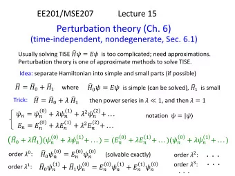
Initial Condition from inflation Inflation gives the initial power spectrum that is nearly a power law. “ ” � n s + 1 k 2 α s ln � k 0 k P ( k, η i ) = A k 0 Inflation predicts, and observations have confirmed, that n s ∼ 1 α s ∼ 0

Initial Power Spectrum: Tilting Initial matter power spectrum for various n s : P ( k ) ∝ ( k/k 0 ) n s

Initial Power Spectrum: Running Initial matter power spectrum for various α s

Evolution of linear perturbations Two key equations The Boltzmann equation d f dλ = C [ f ] Perturbed Einstein’s equations δG µν = 8 πGδT µν Dark Neutrinos energy ρ N ρ N Λ metric Dark Photons mater g µν ρ Θ ρ δ m γ m Compton Compton Scattering Scattering Electrons Baryons ρ δ ρ δ Coulomb Coulomb e e b b Scattering Scattering

Basic equations for linear perturbations The equations for linear perturbations Dark matter δ ′ + ikv = − 3Φ ′ : Continuity v ′ + a ′ a v = − ik Ψ : Euler Baryons b + ikv b = − 3Φ ′ : Continuity δ ′ b + a ′ a v b = − ik Ψ+ τ ′ v ′ R ( v b + 3 i Θ 1 ) : Euler with interaction w/ photons Photon temperature, Θ = ∆ T/T Θ ′ + ikµ Θ = − Φ ′ − ikµ Ψ − τ ′ � Θ 0 − Θ + µv b − 1 � 2 P 2 ( µ )Θ 2 Gravity � � k 2 Φ + 3 a ′ Φ ′ − Ψ a ′ = 4 πGa 2 ( ρ m δ m + 4 ρ r Θ r, 0 ) a a k 2 (Φ + Ψ) = − 32 πGa 2 ρ r Θ r, 2 These are well known equations. Observational test?

Prediction: the CMB power spectrum Sound horizon at the photon decoupling epoch = 147 ± 2 Mpc (Spergel et al. 2007)

WMAP 3-year temperature map 3-year ILC Map (Hinshaw et al., 2007)

Triumph of linear perturbation theory 3-year Temperature Power Spectrum (Hinshaw et al. 2007) Experimental Verification of the Linear Perturbation Theory!

How about the matter P ( k ) ?

SDSS Luminous Red Galaxies map ( z < 0 . 474 ) 1000 500 0 -500 -1000 -1000 -500 0 500 1000 SDSS main galaxies and LRGs (Tegmark et al., 2006)

SDSS LRG and main galaxy power spectrum Failure of linear theory is clearly seen. P ( k ) from main (bottom) and LRGs (top) (Tegmark et al., 2006)

BAO from the SDSS power spectrum The BAOs have been measured in P ( k ) successfully (Percival et al. 2006). The planned galaxy surveys (e.g., HETDEX, WFMOS) will measure BAOs with 10x smaller error bars. Is theory ready?

Systematics: Three Non-linearities The SDSS P ( k ) has been used only up to k < 0 . 1 hMpc − 1 . Why? Non-linearities. Non-linear evolution of matter clustering Non-linear bias Non-linear redshift space distortion Can we do better? CMB theory was ready for WMAP’s precision measurement. LSS theory has not reached sufficient accuracy. The planned galaxy surveys = WMAP for LSS. Is theory ready? The goal: LSS theory that is ready for precision measurements of P ( k ) from the future galaxy surveys.

Our approach: Non-linear perturbation theory 3 rd -order expansion in linear density fluctuations, δ 1 . c.f. CMB theory: 1 st -order (linear) theory. Is this approach new? It has been known that non-linear perturbation theory fails at z = 0 ← − too non-linear. HETDEX ( z > 2 ) and CIP ( z > 3 ) are at higher-z, where perturbation theory is expected to perform better.

Upcoming high-z galaxy surveys

Upcoming high-z galaxy surveys

Assumptions and basic equations Assumptions 1 Newtonian matter fluid 2 Matter is the pressureless fluid without vorticity. Good approximation before fluctuations go fully non-linear. It is convenient to use the “velocity divergence”, θ = ∇ · v Equations (Newtonian one component fluid equation) ˙ δ + ∇ · [(1 + δ ) v ] = 0 v + ( v · ∇ ) v = − ˙ a ˙ a v − ∇ φ ∇ 2 φ = 4 πGa 2 ¯ ρδ

Go to Fourier space Equations in Fourier space ˙ δ ( k , τ ) + θ ( k , τ ) d 3 k 1 � � d 3 k 2 δ D ( k 1 + k 2 − k ) k · k 1 = − δ ( k 2 , τ ) θ ( k 1 , τ ) , (2 π ) 3 k 2 1 a 2 θ ( k , τ ) + ˙ a aθ ( k , τ ) + 3˙ ˙ 2 a 2 Ω m ( τ ) δ ( k , τ ) d 3 k 1 d 3 k 2 δ D ( k 1 + k 2 − k ) k 2 ( k 1 · k 2 ) � � = − θ ( k 1 , τ ) θ ( k 2 , τ ) , (2 π ) 3 2 k 2 1 k 2 2 Taylor expanding δ , and θ ∞ n � (2 π ) 3 · · · d 3 q n − 1 d 3 q 1 � � � a n ( τ ) d 3 q n δ D ( δ ( k , τ ) = q i − k ) F n ( q 1 , q 2 , · · · , q n ) δ 1 ( q 1 ) · · · δ 1 ( q n ) , (2 π ) 3 n =1 i =1 ∞ n (2 π ) 3 · · · d 3 q n − 1 d 3 q 1 � � � a ( τ ) a n − 1 ( τ ) � θ ( k , τ ) = − ˙ d 3 q n δ D ( q i − k ) G n ( q 1 , q 2 , · · · , q n ) δ 1 ( q 1 ) · · · δ 1 ( q n ) (2 π ) 3 n =1 i =1

Why 3 rd order? δ = δ 1 + δ 2 + δ 3 where, δ 2 ∝ [ δ 1 ] 2 , δ 3 ∝ [ δ 1 ] 3 The power spectrum from the higher order density field : (2 π ) 3 P ( k ) δ D ( k + k ′ ) ≡ � δ ( k , τ ) δ ( k ′ , τ ) � = � δ 1 ( k , τ ) δ 1 ( k ′ , τ ) � + � δ 2 ( k , τ ) δ 1 ( k ′ , τ ) + δ 1 ( k , τ ) δ 2 ( k ′ , τ ) � + � δ 1 ( k , τ ) δ 3 ( k ′ , τ ) + δ 2 ( k , τ ) δ 2 ( k ′ , τ ) + δ 3 ( k , τ ) δ 1 ( k ′ , τ ) � + O ( δ 6 1 ) Therefore, P ( k ) = P 11 ( k ) + P 22 ( k ) + 2 P 13 ( k )

Why 3 rd order? δ = δ 1 + δ 2 + δ 3 where, δ 2 ∝ [ δ 1 ] 2 , δ 3 ∝ [ δ 1 ] 3 The power spectrum from the higher order density field : (2 π ) 3 P ( k ) δ D ( k + k ′ ) ≡ � δ ( k , τ ) δ ( k ′ , τ ) � = � δ 1 ( k , τ ) δ 1 ( k ′ , τ ) � + � δ 2 ( k , τ ) δ 1 ( k ′ , τ ) + δ 1 ( k , τ ) δ 2 ( k ′ , τ ) � + � δ 1 ( k , τ ) δ 3 ( k ′ , τ ) + δ 2 ( k , τ ) δ 2 ( k ′ , τ ) + δ 3 ( k , τ ) δ 1 ( k ′ , τ ) � + O ( δ 6 1 ) Therefore, P ( k ) = P 11 ( k ) + P 22 ( k ) + 2 P 13 ( k )

Non-linear matter power spectrum: analytic solution (Vishniac 1983; Fry1984; Goroff et al. 1986;Suto & Sasaki 1991; Makino et al. 1992; Jain & Bertschinger 1994; Scoccimarro & Frieman 1996) P δδ ( k, τ ) = D 2 ( τ ) P L ( k ) + D 4 ( τ ) [2 P 13 ( k ) + P 22 ( k )] , where, d 3 q � � 2 � F ( s ) P 22 ( k ) = 2 (2 π ) 3 P L ( q ) P L ( | k − q | ) 2 ( q , k − q ) , � ∞ 2 πk 2 dq 2 P 13 ( k ) = 252 P L ( k ) (2 π ) 3 P L ( q ) 0 � 100 q 2 k 2 − 158 + 12 k 2 q 2 − 42 q 4 × k 4 � k + q � � 3 k 5 q 3 ( q 2 − k 2 ) 3 (2 k 2 + 7 q 2 ) ln + , | k − q | „ « » – q 2 ) 2 − 1 F ( s ) 2 ( q 1 , q 2 ) = 17 21 + 1 q 1 q 2 + q 2 + 2 2 ˆ q 1 · ˆ q 2 ( ˆ q 1 · ˆ q 1 7 3

Prediction: non-linear matter P(k)

Prediction: Baryon Acoustic Oscillations Non-linearity distorts BAOs significantly.

Simulation Set I: Low-resolution (faster) Particle-Mesh (PM) Poisson solver (Ryu et al. 1993) Cosmological parameters Ω m = 0 . 27 , Ω Λ = 0 . 73 , Ω b = 0 . 043 , H 0 = 70 km / s / Mpc , σ 8 = 0 . 8 , n s = 1 . 0 Simulation parameters Box size [Mpc / h] 3 k max [ h Mpc − 1 ] n particle M particle ( M ⊙ ) N realizations 512 3 256 3 2 . 22 × 10 12 60 0 . 24 256 3 256 3 2 . 78 × 10 11 50 0 . 5 128 3 256 3 3 . 47 × 10 10 20 1 . 4 64 3 256 3 4 . 34 × 10 9 15 5

Testing convergence with 4 box sizes