Perceptron Lecturer: Barnabas Poczos Disclaimer : These notes have - PDF document
Introduction to Machine Learning (Lecture Notes) Perceptron Lecturer: Barnabas Poczos Disclaimer : These notes have not been subjected to the usual scrutiny reserved for formal publications. They may be distributed outside this class only with
Introduction to Machine Learning (Lecture Notes) Perceptron Lecturer: Barnabas Poczos Disclaimer : These notes have not been subjected to the usual scrutiny reserved for formal publications. They may be distributed outside this class only with the permission of the Instructor. 1 History of Artificial Neural Networks The history of artificial neural networks is like a roller-coaster ride. There were times when it was popular(up), and there were times when it wasn’t. We are now in one of its very big time. • Progression (1943-1960) – First Mathematical model of neurons ∗ Pitts & McCulloch (1943) [MP43] – Beginning of artificial neural networks – Perceptron, Rosenblatt (1958) [R58] ∗ A single neuron for classification ∗ Perceptron learning rule ∗ Perceptron convergence theorem [N62] • Degression (1960-1980) – Perceptron can’t even learn the XOR function [MP69] – We don’t know how to train MLP – 1963 Backpropagation (Bryson et al. ) ∗ But not much attention • Progression (1980-) – 1986 Backpropagation reinvented: ∗ Learning representations by back-propagation errors. Rumilhart et al. Nature [RHW88] – Successful applications in ∗ Character recognition, autonomous cars, ..., etc. – But there were still some open questions in ∗ Overfitting? Network structure? Neuron number? Layer number? Bad local minimum points? When to stop training? – Hopfield nets (1982) [H82], Boltzmann machines [AHS85], ..., etc. • Degression (1993-) 1
2 Perceptron: Barnabas Poczos – SVM: Support Vector Machine is developed by Vapnik et al. . [CV95] However, SVM is a shallow architecture. – Graphical models are becoming more and more popular – Great success of SVM and graphical models almost kills the ANN (Artificial Neural Network) research. – Training deeper networks consistently yields poor results. – However, Yann LeCun (1998) developed deep convolutional neural networks (a discriminative model). [LBBH98] • Progression (2006-) Deep learning is a rebranding of ANN research. – Deep Belief Networks (DBN) ∗ A fast learning algorithm for deep belief nets. Hinton et al. Neural Computation. [HOT06] ∗ Generative graphical model ∗ Based on restrictive Boltzmann machines ∗ Can be trained efficiently – Deep Autoencoder based networks ∗ Greedy Layer-Wise Training of Deep Networks.Bengio et al. NIPS [BLPL07] – Convolutional neural networks running on GPUs ∗ Great success for NN since the massiave usage of GPUs. ∗ AlexNet (2012). Krizhevsky et al. NIPS [KSH12] To summarize, in the past, the popularity of artificial neural networks sometimes degraded due to bad per- formance or poor scalability. Recently, thanks to the advancement of computing power (GPUs), availability of big data, and the development of techniques for training deep neural networks on large dataset, artificial neural network and deep learning research have become very popular again. 2 The Neuron • Each neuron has a body, axon, and many dendrites.
Perceptron: Barnabas Poczos 3 • A neuron can fire or rest. • If the sum of weighted inputs is larger than a threshold, then the neuron fires. • Synapses: The gap between the axon and other neuron dendrites. It determines the weights in the sum. 2.1 Mathematical model of a neuron The below figure illustrates the mathematical model of a neuron. Although inspired by biological neurons, this model has a number of simplifications and some of its design may not correspond to the actual function- ality of biological neurons. However, due to its simplicity in computation and its effectiveness in practice, this is one of the most widely-used neuron models nowadays. The output of a neuron y = f ( ω 1 x 1 + . . . + ω n x n ), is computed by applying a transformation f over the weighted sum of the input signals x 1 , x 2 , . . . , x n . The transformation f is called the activation function. The activation function is usually chosen to be non-linear. This allows neural networks to learn complex non-linear transformations over the input signal. Below is a list of different f s that are common. Different activation functions: Identify function: f ( x ) = x Threshold function (perceptron):
4 Perceptron: Barnabas Poczos Ramp function: Logistic function: f ( x ) = (1 + e − x ) − 1 e x + e − x = e 2 x − 1 e 2 x +1 = 1 − e − 2 x Hyperbolic tangent function: f ( x ) = tanh( x ) = e x − e − x 1+ e − 2 x 3 Structure of Neural Networks Neural networks are typically consists of neuron(nodes) and connections(edges). The structure of a neural network refers to the configuration of its neurons and connections. 3.1 An example: Fully connected neural network The network is called fully connected if it has connections between every pair of nodes. It contains input neurons, hidden neurons and output neurons. Each connection has an associated weight as illustrated by the numbers on the edges. There are any models for updating the weights, e.g., asynchronous model. 3.2 Feedforward neural networks Feedforward neural networks are networks that don’t contain backward connections. In other words, messages in feedforward networks are passed layer by layer without feedbacks to previous ones. The connections
Perceptron: Barnabas Poczos 5 between the neurons do not form a cycle. The input layer is conventionally called Layer 0. • There are no connections within the layers • No backward connections • An important special case is the Multilayer perceptron , where there are connections only between Layer i and Layer i + 1 • Most popular architecture • Recurrent NN: there are connections backward. A Matlab demo nnd11nf can visualize these structures. 4 The Perceptron The perceptron is a simple neuron with sgn (threshold) activation function. It can be used to solve simple binary classification problems. Formally it can be described with the following equation: y = sgn ( w T x ) ∈ {− 1 , 1 } . Training set: • X + = { x k | x k ∈ Class + } . • X − = { x k | x k ∈ Class −} . • Assume they are linearly separable.
6 Perceptron: Barnabas Poczos w ∗ is the normal vector of the separating hyperplane through the origin, i.e., w ∗ T x > 0 if x ∈ X + , w ∗ T x < 0 if x ∈ X − . Note If we want to relax the assumption that w ∗ goes through the origin, we could add a bias term b in the vector w ∗ , and add a 1 in the input vecotr X . Our goal is to find such w ∗ . 5 The Perceptron Algorithm Notations Let ˆ y ( k ) denote the predicted label of data x ( k ), which is computed by y ( k ) = sgn ( w ( k − 1) T x ( k ) ˆ Let w ( k ) denote the weight of the k -th iteration. The update rule is given by w ( k ) = w ( k − 1) + µ ( y ( k ) − ˆ y ( k )) x ( k ) The Algorithm 1. Let µ > 0 arbitrary step size parameter. Let w (0) = 0 (it could also be arbitrary) 2. Let k = 1. 3. Let x ( k ) ∈ X + ∪ X − be a training point misclassified by w ( k − 1) 4. If there is no such vector ⇒ 6 5. If ∃ a misclassified vector, then α ( k ) = µǫ ( k ) = µ ( y ( k ) − ˆ y ( k )) w ( k ) = w ( k − 1) + α ( k ) x ( k ) k = k + 1 Back to 3
Perceptron: Barnabas Poczos 7 6. End Observation: If y ( k ) = 1 , ˆ y ( k ) = − 1 , then α ( k ) > 0 . If y ( k ) = − 1 , ˆ y ( k ) = 1 , then α ( k ) < 0 . y ( k )) 2 with learning rate µ : How to remember : Gradient descent on 1 2 ( y ( k ) − ˆ w ( k ) = w ( k − 1) − µ∂ 1 y ( k )) 2 2 ( y ( k ) − ˆ ∂w ( k − 1) An interesting property: we do not require the learning rate to go to zero. (Many learning algorithms requires learning rate to degrade at some point in order to converge) Why the algorithm works? • Each input x i determines a hyperplane orthogonal to x i . • On the + side of the hyperplane for each w ∈ R n : w T x i > 0, sgn ( w T x i ) = 1. • On the − side of the hyperplane for each w ∈ R n : w T x i < 0, sgn ( w T x i ) = − 1. • We need to update the weights, if ∃ x i in the training set, such that sgn ( w T x i ) � = y i , where y i = class ( x i ) ∈ {− 1 , 1 } • Then update w such that ˆ y i gets closer to y i ∈ {− 1 , 1 } Convergence of the Perceptron Algorithm Theorem 1 If the samples are linearly separable, then the perceptron algorithm finds a separating hyperplane in finite steps. Theorem 2 The running time does not depend on the sample size n. Proof Lemma 3 Let X = X + ∪ {− X − } ¯ X we have w ∗ T ¯ x ∈ ¯ Then ∃ b > 0 , such that ∀ ¯ x ≥ b > 0 . Proof: By definition we have that w ∗ T x > 0 if x ∈ X + w ∗ T x < 0 if x ∈ X − .
Recommend
More recommend
Explore More Topics
Stay informed with curated content and fresh updates.




![CS885 Reinforcement Learning Lecture 4a: May 11, 2018 Deep Neural Networks [GBC] Chap. 6, 7, 8](https://c.sambuz.com/940910/cs885-reinforcement-learning-lecture-4a-may-11-2018-s.webp)
