PDE computations often need to use a computational mesh which can - PowerPoint PPT Presentation

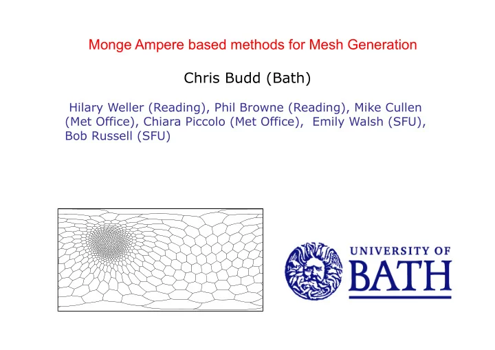
Monge Ampere based methods for Mesh Generation Chris Budd (Bath) Hilary Weller (Reading), Phil Browne (Reading), Mike Cullen (Met Office), Chiara Piccolo (Met Office), Emily Walsh (SFU), Bob Russell (SFU)

PDE computations often need to use a computational mesh which can • Capture small scales and • is aligned with the solution (i) To resolve local geometry eg. orography (ii) For accurate numerical computation of anisotropic evolving features eg. storms, fronts (iii) For accurate approximation of anisotropic functions on many scales eg. For data assimilation calculations

r-adaptive moving mesh methods aim to do this by ‘optimally redistributing’ a fixed number of mesh points Advantages with r-adaptivity • Constant data structures and mesh topology • Ease of coupling to CFD solvers and DA codes • Capturing dynamical physics of the solution eg. symmetries, conservation laws, self-similarity • Global and Local control of mesh regularity eg. Good alignment properties, anisotropic meshes, small scales Traditional problems with r-adaptivity eg. Mesh tangling, mesh skewness, implementation in 3D Can be overcome with suitably designed methods

Eg. Solution of the Eady equations [Cullen]

Geometrical strategy r-adaptive methods are equivalent to MAPS Have a computational domain Ω C ( ξ , η , ς ) Physical domain Ω P ( x , y , z ) Map: J = ∂ ( x , y , z ) F ( t ) : Ω C ( ξ , η , ς ) → Ω P ( x , y , z ), ∂ ( ξ , η , ς )

Most r-adaptive methods define a solution scale m ( x , y , z ) > 0 Unit measure in the physical domain controls the mesh density A: unit set in computational domain F(A,t) : image set Equidistribute integral with respect to this measure ∫ ξ d η d ς = ∫ d m ( x , y , z , t ) dx dy dz A F ( A ) Equidistribution minimises the maximum value of this integral

Differentiate to give: m ( x , y , z , t ) det( J ) = 1 Basic, nonlinear, equidistribution mesh equation Choose the scalar function m To concentrate points where needed without depleting points elsewhere: Eg. m can be truncation error/physics/scaling

Mesh construction 1D: Mesh is completely defined by local scaling (equidistribution) 2D and 3D Need additional conditions to define the mesh uniquely: Local: Mesh alignment [Huang], mesh orthogonality [Thompson], lack of skewness [many] Global: Mesh regularity, avoidance of mesh tangling Argue: A good mesh for solving a PDE is often one which is as close as possible to a uniform mesh

Optimally transported meshes (Monge-Kantorovich) 2 d ξ d η d ς Minimise ∫ I ( x , y , z ) = ( x , y , z ) − ( ξ , η , ς ) Ω C m ( x , y , z , t ) ∂ ( x , y , z ) Subject to ∂ ( ξ , η , ς ) = 1 Optimal transport: global regularity condition • reduces mesh skewness (local!!) • prevents mesh tangling • gives good mesh alignment (local!!) • is effective in generating anisotropic meshes

Key result! Theorem: [Brenier] (a) There exists a unique optimally transported mesh (b) For such a mesh the map F is the gradient of a convex function P ( ξ , η , ς ) P : Scalar mesh potential ( x , y , z ) = ( P ξ , P η , P ς ) J ≡ ∂ ( x , y , z ) T + λ 2 e 2 e 2 T , is symmetric J = λ 1 e 1 e 1 e 1 ⊥ e 2 ∂ ( ξ , η , ς ) ∇ × ( x , y , z ) = 0 Irrotational mesh (avoids tangling)

It follows immediately in 2D that $ ' P P ξξ ξη ηη − P 2 J = H ( P ) = det ) = P ξξ P & ξη P P % ( ξη ηη Hence the mesh equidistribution equation becomes m ( ∇ P , t ) H ( P ) = 1 (MA) Monge-Ampere equation Augment with nonlinear Neumann or periodic boundary conditions to map boundaries to boundaries Solve in parallel with the solution of the underlying PDE

Solution method 1: Use relaxation in n Dimensions 1/ n ( ) Q t = m ( ∇ Q ) H ( Q ) ( ) ε I − α Δ ξ Spatial smoothing Ensures right-hand- Smoothed Invert operator side scales like Q in monitor using a spectral nD to give global method existence Parabolic Monge-Ampere equation (PMA)

Implementation [Browne] If M is prescribed then the PMA equation can be discretised on N points in the computational domain and solved using an explicit forward Euler method with a suitably small timestep, coupled to a fast spectral solver for the smoothing term This is a fast procedure: 5 mins for a full 3D meteorological mesh. Scales as O(N log(N)) Locally we can prove that provided the time step for the iteration is sufficiently small || ∇ Q − ∇ P || < Ce − at 1. Q converges to P exponentially fast 2. Q remains convex at all times, avoiding mesh tangling.

Eg 1: A 3d spherical shell

Convergence history Exponentially fast convergence CPU cost is proportional to N log(N)

Eg 2. Operational mesh calculation for meteorological data assimilation Frontal system: Rain storm in SW UK

Take m to be a scaled approximation of the Potential Vorticity of the 3D flow Coupled to 1d DA procedure [Piccolo, Cullen, Browne]

Eg 3: Buckley-Leverett equation (gas dynamics) F ( u ) = u 2 /( u 2 + (1 − u ) 2 ), u t = − F x − G y + µ ∇ 2 u , G ( u ) = (1 − 5(1 − u ) 2 ) F Solve using simultaneous mesh and solution calculation with m the solution arc-length

Mesh Regularity: 1. Alignment The meshes generated align perfectly to a linear features J = U T Λ U U: rotation of the linear feature U = [ e 1 e 2 ] e 1 ⊥ e 2 Anisotropy can be estimated from solving MA and is beneficial

Also align to radial features: Exact solution of the MA equation x = ξ R ( r ) y = η R ( r ) ξ 2 + η 2 , a i r 2 − b i 2 , , , r = R ( r ) = i = 1,2,3 r r Analytic solution Solution close to identity for large r or R

Example: Radially symmetric singularity at the origin Leaf-like structure away from the Very uniform close to singularity the singularity

Mesh regularity: 2. Skewness in 2d Skewness measure Can calculate exactly for particular solutions of Monge- Ampere which represent important features

Solution 2: Fixed point iteration [Weller] Plane: Use Laplacian preconditioning to give a fixed point iteration Discretise using a finite volume method and algebraic multigrid to solve for the Laplacian

Monitor function: min = 0.015586 max = 0.99929 0.0 0.1 0.2 0.3 0.4 0.5 0.6 0.7 0.8 0.9 1.0

Can extend to the surface of the sphere: [Weller] Sphere: Maps along the geodesic parallel to ∇ φ φ r( ) Ratio of volumes of original cells to the final cells Iteration (on the surface of the sphere):

Mesh on sphere with m = precipitation density

Next steps: • Rigorous proofs of error estimates of anisotropic meshes • Coupling to hyperbolic PDEs using semi-Lagrangian methods • Extend to mimetic finite elements on the sohere • Application to seriously large problems

Conclusions • Optimal transport is a natural way to determine moving meshes • Method works well for a variety of problems, and there are rigorous estimates about its behaviour • Provable alignment properties • Excellent for interpolation .. • Coupling to PDE still a big issue

Skewness for a very singular solution 0.5 7 0.4 0.4 6 0.3 0.3 0.2 0.2 5 0.1 0.1 0 y 0 4 y − 0.1 − 0.1 3 − 0.2 − 0.2 − 0.3 − 0.3 2 − 0.4 − 0.4 − 0.5 1 − 0.5 0 0.5 − 0.4 − 0.3 − 0.2 − 0.1 0 0.1 0.2 0.3 0.4 x x