PCA: algorithm 6. Project each point onto the eigenspace, giving a - - PowerPoint PPT Presentation

PCA: algorithm

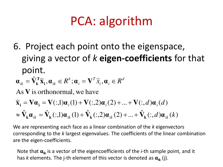
• 6. Project each point onto the eigenspace,

giving a vector of k eigen-coefficients for that point.

) ( ) (:, ˆ ... ) 2 ( ) 2 (:, ˆ ) 1 ( ) 1 (:, ˆ ˆ ) ( ) (:, ... ) 2 ( ) 2 (:, ) 1 ( ) 1 (:, have we l,

• rthonorma

is As , ; , ˆ k d d d R x R

ik ik ik ik i i i d i i T i k ik ik

α V α V α V α V α V α V α V Vα x V α V α α x V α

k k k k i i i T k

+ + + = ≈ + + + = = ∈ = ∈ =

We are representing each face as a linear combination of the k eigenvectors corresponding to the k largest eigenvalues. The coefficients of the linear combination are the eigen-coefficients. Note that αik is a vector of the eigencoefficients of the i-th sample point, and it has k elements. The j-th element of this vector is denoted as αik (j).

PCA: Algorithm

• 1. Compute the mean of the given points:
• 2. Deduct the mean from each point:
• 3. Compute the covariance matrix of these

mean-deducted points:

d d i N i i

R R N ∈ ∈ =

∑

=

x x x x , , 1

1

x x x

i i

− = te semidefini

• positive

is it and matrix, symmetric a is : : , 1 1 1 1

1 1

C C ) x )(x x (x x x C

i i

Note R Note N N

d d N i T T i N i i × = =

∈ − − − = − =

∑ ∑

PCA: algorithm

• 4. Find the eigenvectors of C:
• 5. Extract the k eigenvectors corresponding to the k

largest eigenvalues. This is called the extracted eigenspace:

values)

• (eigen

diagonal

• n the

values negative

• non

contains : symmetric. is it hence and matrix covariance a is as ), (i.e. matrix l

• rthonorma

an is : s eigenvalue

• f

matrix diagonal r), eigenvecto an is column (each rs eigenvecto

• f

matrix , , Λ C I V V VV V Λ V Λ V VΛ CV Note Note R R

T T d d d d

= = − − ∈ ∈ =

× ×

) : 1 (:, ˆ k V Vk =

There is an implicit assumption here that the first k indices indeed correspond to the k largest eigenvalues. If that is not true, you would need to pick the appropriate indices.

PCA and Face Recognition: Eigen-faces

• Consider a database of cropped, frontal face images (which we

will assume are aligned and under the same illumination). These are the gallery images.

• We will reshape each such image (a 2D array of size H x W after

cropping) to form a column vector of d = HW elements. Each image will be a vector xi, as per the notation on the previous two slides.

• And then carry out the six steps mentioned before.
• The eigenvectors that we get in this case are called eigenfaces.

Each eigenvector has d elements. If you reshape those eigenvectors to form images of size H x W, those images look like (filtered!) faces.

Example 1

A face database http://people.ece.cornell.edu/land/courses/ece4760/FinalProjects/s2011/bjh78_caj65/b jh78_caj65/

Top 25 Eigen-faces for this database! http://people.ece.cornell.edu/land/courses/ece4760/FinalProjects/s2011/bjh78_caj65/b jh78_caj65/

One word of caution: Eigen-faces

• The algorithm described earlier is

computationally infeasible for eigen-faces, as it requires storage of a d x d Covariance matrix (d – the number of image pixels - could be more than 10,000). And the computation of the eigen- vectors of such a matrix is a O(d3) operation!

• We will study a modification to this that will bring

down the computational cost drastically.

Eigen-faces: reducing computational complexity.

• In such a case, the rank of C is at the most N-1.

So C will have at the most N-1 non-zero eigen- values.

• We can write C in the following way:

N d T T i N i i

R N

× =

∈ = ∝ − =

∑

] x | ... | x | x [ X XX x x C

N 2 1

where , 1 1

1

Back to Eigen-faces: reducing computational complexity.

• Consider the matrix XTX (size N x N) instead of

XXT (size d x d). Its eigenvectors are of the form:

] by g multiplyin pre )[ ( ) ( , X Xw Xw XX w w Xw X − = → ∈ = λ λ

T N T

R

Xw is an eigenvector of C=XXT! Computing all eigenvectors of C will now have a complexity of only O(N3) for computation of the eigenvectors of XTX + O(N x dN) for computation of Xw from each w = total of O(N3 + dN2) which is much less than O(d3). Note that C has at most only min(N- 1,d) eigenvectors corresponding to non-zero eigen-values (why?).

Eigenfaces: Algorithm (N << d case)

• 1. Compute the mean of the given points:
• 2. Deduct the mean from each point:
• 3. Compute the following matrix:

te semidefini

• positive

is it and matrix, symmetric a is : ] [ , , L x | ... | x | x X L X X L

N 2 1

Note R R

N d N N T × ×

∈ = ∈ =

d d i N i i

R R N ∈ ∈ =

∑

=

x x x x , , 1

1

x x x

i i

− =

Eigen-faces: Algorithm (N << d case)

• 4. Find the eigenvectors of L:
• 5. Obtain the eigenvectors of C from those of L:
• 6. Unit-normalize the columns of V.
• 7. C will have at most only N eigenvectors corresponding

to non-zero eigen-values*. Out of these you pick the top k (k < N) corresponding to the largest eigen-values. * Actually this number is at most N-1 – this is due to the mean subtraction, else it would have been at most N.

I WW Γ W WΓ LW = − − =

T

s eigenvalue rs eigenvecto , , ,

N N N N N d

R R R

× × ×

∈ ∈ ∈ = V W X XW V , , ,

Top 25 eigenfaces from the previous database Reconstruction of a face image using the top 1,8,16,32,…,104 eigenfaces (i.e. k varied from 1 to 104 in steps of 8)

∑

=

+ ≈ + =

k l

l l

1

) ( ) (:, ˆ ˆ

ik i i

α V x α V x x

Example 2

The Yale Face database

What if both N and d are large?

• This can happen, for example, if you wanted

to build an eigenspace for face images of all people in Mumbai.

• Divide people into coherent groups based on

some visual attributes (eg: gender, age group etc) and build separate eigenspaces for each group.

PCA: A closer look

• PCA has many applications – apart from

face/object recognition – in image processing/computer vision, statistics, econometrics, finance, agriculture, and you name it!

• Why PCA? What’s special about PCA? See the

next slides!

PCA: what does it do?

• It finds ‘k’ perpendicular directions (all passing

through the mean vector) such that the

• riginal data are approximated as accurately

as possible when projected onto these ‘k’ directions.

• We will see soon why these ‘k’ directions are

eigenvectors of the covariance matrix of the data!

PCA

Look at this scatter-plot of points in 2D. The points are highly spread out in the direction of the light blue line.

PCA

This is how the data would look if they were rotated in such a way that the major axis of the ellipse (the light blue line) now coincided with the Y axis. As the spread of the X coordinates is now relatively insignificant (observe the axes!), we can approximate the rotated data points by their projections onto the Y-axis (i.e. their Y coordinates alone!). This was not possible prior to rotation!

PCA

• Aim of PCA: Find the line passing through

the sample mean (i.e. ), such that the projection of any mean-deducted point

• nto , most accurately approximates it.

x x xi −

e 

) x

• ( x

e e e x

• x

i T i i i i

   = ∈ = a a a , , is

• nto
• f

Projection R

2

ion approximat

• f

Error ) x ( x ) e ( a

i i

− − = 

xi

x e 

ai

x xi −

Note: Here is a unit vector.

e 

e 

PCA

• Summing up over all points, we get:

∑

=

− − = =

N i i

a J

1 2

) ( ) ( ) ( ion approximat

• f

error total Sum x x e e

i

  ) ( 2

1 1 2 1 2

x x e x x

i i

− − − + =

∑ ∑ ∑

= = = T N i i N i N i i

a a  ) ( 2 ) (

1 1 2 1 2

x x e x x e

i i

− − − + =

∑ ∑ ∑

= = = T N i i N i N i i

a a   ) ( 2 ) (

1 1 2 1 2

x x e x x e

i i

− − − + =

∑ ∑ ∑

= = = T N i i N i N i i

a a  

∑ ∑ ∑ ∑ ∑

= = = = =

− + − = − = − − + =

N i N i i T i N i i N i N i i

a a a a

1 2 1 2 1 2 1 2 1 2

)) ( ( , 2 x x x x e x x

i i i

 

PCA

∑ ∑

= =

− + − = =

N i N i i

a J

1 2 1 2

) ( ion approximat

• f

error total Sum x x e

i



This term is proportional to the variance of the data points when projected onto the direction e.

∑ ∑

= =

− + − − − =

N i N i t t 1 2 1

) )( ( x x e x x x x e

i i i

 

∑ ∑

= =

− + − − =

N i N i t 1 2 1 2

)) ( ( x x x x e

i i

 ) ) 1 ( where (

1 2

C S x x e S e

i

− = − + − =

∑

=

N

N i t

 

PCA

.

• f

eigenvalue maximum the to ing correspond vector

• eigen

the be to choose we , maximize to wish we and As .

• f

vector

• eigen

an is so , get we , it to setting and w.r.t. ) ( ~

• f

derivative Taking ( ) ( ~ 0) it to set (and w.r.t. function modified following the

• f

derivative the take to have we So . 1 that constraint the imposing usly simultaneo while so, do to s multiplier Lagrange

• f

method the use We . w.r.t. maximizing to equivalent is w.r.t. Minimizing ) (

1 2

S e e S e e S e S e e e S e e 1) 1)

• e

e e S e e e e e e S e e e x x e S e e

t t i t

                         

t t t t N i

J e J ) J( J λ λ λ = = − = = − + − =

∑

=

Independent of the direction e See appendix for details

PCA

• PCA thus projects the data onto that direction

that minimizes the total squared difference between the data-points and their respective projections along that direction.

• This equivalently yields the direction along which

the spread (or variance) will be maximum.

• Why? Note that the eigenvalue of a covariance

matrix tells you the variance of the data when projected along that particular eigenvector:

∑

=

− = = → =

N i t t t 1 2

)) ( ( x xi e e S e e S e e e S        λ λ

This term is proportional to the variance of the data when projected along e.

PCA

• But for most applications (including face recognition), just a

single direction is absolutely insufficient!

• We will need to project the data (from the high-

dimensional, i.e. d-dimensional space) onto k (k << d) different mutually perpendicular directions.

• What is the criterion for deriving these directions?
• We seek those k directions for which the total

reconstruction error of all the N images when projected on those directions is minimized.

PCA

• We seek those k directions for which the total

reconstruction error of all the N images when projected on those directions is minimized.

• One can prove that these k directions will be the

eigenvectors of the S matrix (equivalently covariance matrix

• f the data) corresponding to the k-largest eigenvalues.

These k directions form the eigen-space.

• If the eigenvalues of S are distinct, these k directions are

defined uniquely (up to a sign factor)

2 2 1 1 1

)) ( ) ( ) } ({

∑ ∑

= = =

− − − =

N i k j t k j

J

j i j i j

e x x (e x x e

PCA

• One can prove that these k directions will be the eigenvectors of

the S matrix (equivalently covariance matrix of the data) corresponding to the k-largest eigenvalues. These k directions form the eigen-space.

• Sketch of the proof:

 Assume we have found e1 and are looking for e2 (where e2 is perpendicular to e1 and e2 has unit magnitude).  Write out the objective function with the two constraints.  Minimize it and do some algebra to see that e2 is the eigenvector

• f S with the second largest eigenvalue.

 Proceed similarly for other directions.

The eigenvalues of the covariance matrix typically decay fast in value (if the faces were properly normalized). Note that the j-th eigenvalue is proportional to the variance of the j-th eigencoefficient, i.e.

) ( ) 1 ( ) )( (

2 1 ij N i t j

E N α λ − = − − = =

∑

= j i i t j j t j

e x x x x e Se Se e

What this means is that the data have low variance when projected along most of the eigenvectors, i.e. effectively the data are concentrated in a lower-dimensional subspace of the d-dimensional space.

PCA: Compression of a set of images

• Consider a database of N images that are

“similar” (eg: all are face images, all are car images, etc.)

• Build an eigen-space from some subset of

these images (could be all images, as well)

• We know that these images can often be

reconstructed very well (i.e. with low error) using just a few eigenvectors.

PCA: Compression of a set of images

• Use this fact for image compression.
• Original data storage = d pixels x N images = Nd bytes

(assume one byte per pixel intensity) = 8Nd bits.

• After PCA: Nk x number of bits to store each eigen-

coefficient = 32Nk bits (remember k << d, example: d ~ 250,000 and k ~ 100).

• Plus storage of eigenvectors = 32dk bits (remember k

<< M as well).

• Plus mean image = 8d bits.
• Total: 32(N+d)k + 8d bits

PCA: Compression of a set of images

• Example: N= 5000, d = 250000, k = 100
• Original size/(size after PCA compression) ~

12.2.

• Note: we allocated 32 bits for every element
• f the eigen-vector. This is actually very

conservative and you can have further savings using several tricks.

Which is the best orthonormal basis? Relationship between PCA and DCT

• Consider a set of M data-points (e.g. image

patches in a vectorized form) represented as a linear combination of column vectors of an

• rtho-normal basis matrix:
• Suppose we reconstruct each patch using only

a subset of some k coefficients as follows:

I U U UU UU θ q U θ q = = ∈ ∈ =

× × T T N i N i i i

R R , , ,

1 1

patches) all for retained are ts coefficien same (the ts coefficien except all to setting by

• btained

is ~ where , ~ ~

) (

k k

i i k i

θ θ U q =

Which is the best orthonormal basis? Relationship between PCA and DCT

• For which orthonormal basis U is the following

error the lowest:

∑

=

− =

M i i k i

E

1 2 ) (

~ ) ( q q U

Which is the best orthonormal basis? Relationship between PCA and DCT

• The answer is the PCA basis, i.e. the set of k

eigenvectors of the correlation matrix C, corresponding to the k largest eigen-values. Here is C is defined as:

ilk M i ikl kl T i M i i

q q M C M

∑ ∑

= =

− = − =

1 1

1 1 , 1 1 q q C

PCA: separable 2D version

• Find the correlation matrix CR of row vectors from

the patches.

• Find the correlation matrix CC of column vectors

from the patches.

• The final PCA basis is the Kronecker product of the

individual bases:

n n n n n n n n T th n i M i n j i i th n i M i n j i i

R R R R I j R j q eig j q j q M j R j q eig j q j q M

× × × × × = = × = =

∈ ∈ ∈ ∈ = ⊗ = − ∈ = − = − ∈ = − =

∑∑ ∑∑

i C R C R i C C C C i R R R R

q V V V VV VV V V V q C D , V C q C D , V C , , , ; ;

• f

vector column ) (:, ); ( ] [ ; )' (:, ) (:, 1 1

• f

row vector :) , ( ); ( ] [ ; :) , ( :)' , ( 1 1

2 2

1 1 1 1 1 1

Experiment

• Suppose you extract M ~ 100,000 small-sized (8 x 8) patches from a set of

images.

• Compute the column-column and row-row correlation matrices.
• Compute their eigenvectors VR and VC.
• The eigenvectors will be very similar to the columns of the 1D-DCT matrix!

(as evidenced by dot product values).

• Now compute the Kronecker product of VR and VC and call it V. Reshape

each column of V to form an image. These images will appear very similar to the DCT bases.

∑∑ ∑ ∑∑ ∑

= = = = = =

− = − = − = − =

M i j i i i M i T i M i j i i M i T i i

j P j P M M j P j P M M

1 8 1 1 1 8 1 1

:); , ( :)' , ( 1 1 1 1 ; )' (:, ) (:, 1 1 1 1 P P C P P C

R C

Code: https://www.cse.iitb.ac.in/~ajitvr/CS663_Fall2017/dct_pca.m

0.3536 0.4904 0.4619 0.4157 0.3536 0.2778 0.1913 0.0975 0.3536 0.4157 0.1913 -0.0975 -0.3536 -0.4904 -0.4619 -0.2778 0.3536 0.2778 -0.1913 -0.4904 -0.3536 0.0975 0.4619 0.4157 0.3536 0.0975 -0.4619 -0.2778 0.3536 0.4157 -0.1913 -0.4904 0.3536 -0.0975 -0.4619 0.2778 0.3536 -0.4157 -0.1913 0.4904 0.3536 -0.2778 -0.1913 0.4904 -0.3536 -0.0975 0.4619 -0.4157 0.3536 -0.4157 0.1913 0.0975 -0.3536 0.4904 -0.4619 0.2778 0.3536 -0.4904 0.4619 -0.4157 0.3536 -0.2778 0.1913 -0.0975

DCT matrix: dctmtx command from MATLAB (see code on website)

0.3517 -0.4493 -0.4278 0.4230 0.3754 0.3247 -0.2250 -0.1245 0.3534 -0.4366 -0.2276 -0.0110 -0.3078 -0.4746 0.4732 0.2975 0.3543 -0.3101 0.1728 -0.4830 -0.3989 0.0498 -0.4299 -0.4109 0.3546 -0.1115 0.4799 -0.3005 0.3342 0.4102 0.1856 0.4761 0.3547 0.1141 0.4823 0.2944 0.3301 -0.4182 0.1745 -0.4771 0.3543 0.3104 0.1771 0.4834 -0.3977 -0.0322 -0.4308 0.4103 0.3535 0.4357 -0.2319 0.0143 -0.3009 0.4656 0.4851 -0.2975 0.3520 0.4468 -0.4328 -0.4204 0.3686 -0.3253 -0.2342 0.1261 0.3520 -0.4461 -0.4305 0.4224 0.3696 0.3247 0.2342 0.1283 0.3537 -0.4338 -0.2345 -0.0114 -0.3000 -0.4671 -0.4814 -0.3028 0.3545 -0.3086 0.1662 -0.4896 -0.4007 0.0359 0.4261 0.4102 0.3548 -0.1145 0.4763 -0.3031 0.3339 0.4198 -0.1800 -0.4713 0.3548 0.1056 0.4839 0.2926 0.3349 -0.4194 -0.1766 0.4733 0.3543 0.3043 0.1863 0.4833 -0.4028 -0.0354 0.4269 -0.4097 0.3532 0.4389 -0.2269 0.0180 -0.3008 0.4654 -0.4811 0.3037 0.3512 0.4562 -0.4300 -0.4126 0.3694 -0.3242 0.2335 -0.1319

VC: Eigenvectors of column- column correlation matrix VR: Eigenvectors of row-row correlation matrix

1.0000 0.0007 0.0032 0.0002 0.0013 0.0001 0.0005 0.0000 0.0007 0.9970 0.0097 0.0689 0.0009 0.0322 0.0003 0.0110 0.0033 0.0106 0.9968 0.0118 0.0713 0.0004 0.0334 0.0025 0.0002 0.0718 0.0124 0.9926 0.0007 0.0927 0.0017 0.0276 0.0010 0.0001 0.0737 0.0004 0.9942 0.0008 0.0780 0.0010 0.0000 0.0261 0.0015 0.0962 0.0005 0.9934 0.0011 0.0569 0.0003 0.0007 0.0276 0.0021 0.0802 0.0010 0.9964 0.0013 0.0000 0.0076 0.0026 0.0227 0.0012 0.0596 0.0015 0.9979 1.0000 0.0002 0.0029 0.0001 0.0010 0.0000 0.0004 0.0000 0.0002 0.9965 0.0028 0.0766 0.0005 0.0314 0.0009 0.0107 0.0029 0.0025 0.9969 0.0046 0.0728 0.0017 0.0304 0.0013 0.0001 0.0795 0.0044 0.9923 0.0029 0.0916 0.0015 0.0243 0.0008 0.0003 0.0747 0.0026 0.9948 0.0061 0.0696 0.0004 0.0000 0.0246 0.0021 0.0949 0.0069 0.9940 0.0131 0.0452 0.0003 0.0004 0.0252 0.0003 0.0715 0.0137 0.9970 0.0002 0.0000 0.0076 0.0013 0.0207 0.0001 0.0476 0.0009 0.9986

Absolute value of dot products between the columns of DCT matrix and columns of VR (left) and VC (right)