Partitioning Decompose computation into tasks to equi-distribute the - PowerPoint PPT Presentation
Lecture 12: Partitioning and Load Balancing G63.2011.002/G22.2945.001 November 16, 2010 thanks to Schloegel,Karypis and Kumar survey paper and Zoltan website for many of todays slides and pictures Partitioning Decompose
Lecture 12: Partitioning and Load Balancing ∗ G63.2011.002/G22.2945.001 · November 16, 2010 ∗ thanks to Schloegel,Karypis and Kumar survey paper and Zoltan website for many of today’s slides and pictures
Partitioning • Decompose computation into tasks to equi-distribute the data and work, minimize processor idle time. applies to grid points, elements, matrix rows, particles, VLSI layout, ,... • Map to processors to keep interprocessor communication low. communication to computation ratio comes from both the partitioning and the algorithm.
Partitioning Data decomposition + Owner computes rule: • Data distributed among the processors • Data distribution defines work assignment • Owner performs all computations on its data. • Data dependencies for data items owned by different processors incur communication
Partitioning • Static - all information available before computation starts use off-line algorithms to prepare before execution time; run as pre-processor, can be serial, can be slow and expensive, starts. • Dynamic - information not known until runtime, work changes during computation (e.g. adaptive methods), or locality of objects change (e.g. particles move) use on-line algorithms to make decisions mid-execution; must run side-by-side with application, should be parallel, fast, scalable. Incremental algorithm preferred (small changes in input result in small changes in partitions) will look at some geometric methods, graph-based methods, spectral methods, multilevel methods, diffusion-based balancing,...
Recursive Coordinate Bisection Divide work into two equal parts using cutting plane orthogonal to coordinate axis For good aspect ratios cut in longest dimension. 1st cut 3rd 3rd 2nd 2nd 3rd 3rd Parallel Volume Renderin Can generalize to k-way partitions. Finding optimal partitions is NP hard. (There are optimality results for a class of graphs as a graph partitioning problem.)
Recursive Coordinate Bisection + Conceptually simple, easy to implement, fast. + Regular subdomains, easy to describe – Need coordinates of mesh points/particles. – No control of communication costs. – Can generate disconnected subdomains
Recursive Coordinate Bisection Implicitly incremental - small changes in data result in small movement of cuts
Recursive Inertial Bisection For domains not oriented along coordinate axes can do better if account for the angle of orientation of the mesh. Use bisection line orthogonal to principal inertial axis (treat mesh elements as point masses). Project centers-of-mass onto this axis; bisect this ordered list. Typically gives smaller subdomain boundary.
Space-filling Curves Linearly order a multidimensional mesh (nested hierarchically, preserves locality) Peano-Hilbert ordering Morton ordering
Space-filling Curves Easily extends to adaptively refined meshes 5 6 11 12 15 16 3 4 7 10 13 14 17 19 18 8 2 9 20 21 25 22 26 24 23 1 27 28
Space-filling Curves 100 1 25 50 75 Partition work into equal chunks.
Space-filling Curves + Generalizes to uneven work loads - incorporate weights. + Dynamic on-the-fly partitioning for any number of nodes. + Good for cache performance
Space-filling Curves – Red region has more communication - not compact – Need coordinates
Space-filling Curves Generalizes to other non-finite difference problems, e.g. particle methods, patch-based adaptive mesh refinement, smooth particle hydro.,
Space-filling Curves Implicitly incremental - small changes in data results in small movement of cuts in linear ordering
Graph Model of Computation • for computation on mesh nodes, graph of the mesh is the graph of the computation; if there is an edge between nodes there is an edge between the vertices in the graph. • for computation on the mesh elements the element is a vertex; put an edge between vertices if the mesh elements share an edge . This is the dual of the node graph.
Graph Model of Computation • for computation on mesh nodes, graph of the mesh is the graph of the computation; if there is an edge between nodes there is an edge between the vertices in the graph. • for computation on the mesh elements the element is a vertex; put an edge between vertices if the mesh elements share an edge . This is the dual of the node graph. Partition vertices into disjoint subdomains so each has same number. Estimate total communication by counting number of edges that connect vertices in different subdomains (the edge-cut metric).
Greedy Bisection Algorithm (also LND) Put connected components together for min communication. • Start with single vertex (peripheral vertex, lowest degree, endpoints of graph diameter) • Incrementally grow partition by adding adjacent vertices (bfs) • Stop when half the vertices counted (n/p for p partitions)
Greedy Bisection Algorithm (also LND) Put connected components together for min communication. • Start with single vertex (peripheral vertex, lowest degree, endpoints of graph diameter) • Incrementally grow partition by adding adjacent vertices (bfs) • Stop when half the vertices counted (n/p for p partitions) + At least one component connected – Not best quality partitioning; need multiple trials.
Breadth First Search • All edges between nodes in same level or adjacent levels. • Partitioning the graph into nodes < = level L and > = L+1 breaks only tree and interlevel edges; no ”extra” edges.
Breadth First Search BFS of two dimensional grid starting at center node.
Graph Partitioning for Sparse Matrix Vector Mult. Compute y = Ax , A sparse symmetric matrix, Vertices v i represent x i , y i . Edge (i,j) for each nonzero A ij Black lines represent communication.
Graph Partitioning for Sparse Matrix Factorization Nested dissection for fill-reducing orderings for sparse matrix factorizations. Recursively repeat: • Compute vertex separator, bisect graph, edge separator = smallest subset of edges such that removing them divided graph into 2 disconnected subgraphs) vertex separator = can extend edge separator by connecting each edge to one vertex, or compute directly. • Split a graph into roughly equal halves using the vertex separator At each level of recursion number the vertices of the partitions, number the separator vertices last. Unknowns ordered from n to 1. Smaller separators ⇒ less fill and less factorization work
Spectral Bisection Gold standard for graph partitioning (Pothen, Simon, Liou, 1990) Let � − 1 i ∈ A ( x i − x j ) 2 = 4 · # cut edges � x i = 1 i ∈ B ( i , j ) ∈ E Goal: find x to minimize quadratic objective function (edge cuts) for integer-valued x = ± 1. Uses Laplacian L of graph G: d ( i ) i = j l ij = − 1 i � = j , ( i , j ) ∈ E 0 otherwise
Spectral Bisection 1 − 1 − 1 2 0 0 4 − 1 2 0 0 − 1 L = − 1 0 3 − 1 − 1 = D − A 2 5 0 0 − 1 1 0 0 − 1 − 1 0 2 3 • A = adjacency matrix; D diagonal matrix • L is symmetric, so has real eigenvalues and orthogonal evecs. • Since row sum is 0, Le = 0, where e = ( 111 . . . 1 ) t • Think of second eigenvector as first ”vibrational” mode
Spectral Bisection Note that n � � � x t Lx = x t Dx − x t Ax = d i x 2 ( x i − x j ) 2 i − 2 x i x j = i = 1 ( i , j ) ∈ E ( i , j ) ∈ E x 2 + x 3 x 1 + x 5 x t Ax = ( x 1 x 2 x 3 x 4 x 5 ) Using previous example, x 1 + x 4 + x 5 x 3 + x 4 x 2 + x 3 + x 5 So finding x to minimize cut edges looks like minimizing x t Lx over vectors x = ± 1 and � n i = 1 x i = 0 (balance condition).
Spectral Bisection • Integer programming problem difficult. • Replace x i = ± 1 with � n i = 1 x 2 i = n x t Lx x t min = 2 Lx 2 � x i = 0 � x 2 i = n λ 2 x t = 2 · x 2 = λ 2 n • λ 2 is the smallest positive eval of L, with evec x 2 , (assuming G is connected, λ 1 = 0 , x 1 = e ) • x 2 satisfies � x i = 0 since orthogonal to x 1 , e t x 1 = 0 • x 2 called Fiedler vector (properties studied by Fiedler in 70’s).
Spectral Bisection • Assign vertices according to the sign of the x 2 . Almost always gives connected subdomains, with significantly fewer edge cuts than RCB. (Thrm. (Fiedler) If G is connected, then one of A,B is. If ∄ i , x 2 i = 0 then other set is connected too). • Recursively repeat (or use higher order evecs) 1 4 . 256 . 437 2 v 2 = − . 138 5 − . 811 3 . 256
Spectral Bisection + High quality partitions – How find second eval and evec? (Lanczos, or CG, .... how do this in parallel, when you don’t yet have the partition?)
Kernighan-Lin Algorithm • Heuristic for graph partitioning (even 2 way partitioning with unit weights is NP complete) • Needs initial partition to start, iteratively improve it by making small local changes to improve partition quality (vertex swaps that decrease edge-cut cost) 1 1 5 5 8 8 2 2 7 7 3 3 6 6 4 4 cut cost 4 cut cost 2
Recommend
More recommend
Explore More Topics
Stay informed with curated content and fresh updates.
