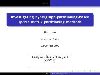
Partitioning for applications Outline Meshes Rob H. Bisseling, - PowerPoint PPT Presentation
Partitioning for applications Outline Meshes Rob H. Bisseling, Albert-Jan Yzelman, Bas Fagginger Auer Laplacian BSP cost Diamonds Mathematical Institute, Utrecht University 3D Rob Bisseling: also joint Laboratory CERFACS/INRIA, Toulouse,
Partitioning for applications Outline Meshes Rob H. Bisseling, Albert-Jan Yzelman, Bas Fagginger Auer Laplacian BSP cost Diamonds Mathematical Institute, Utrecht University 3D Rob Bisseling: also joint Laboratory CERFACS/INRIA, Toulouse, May–July Matrices 2010 Matrix-vector Movies Hypergraphs SBD Mesh-Matrix Conclusions Albert-Jan Bas CERFACS Seminar Toulouse, July 13, 2010 1
Mesh partitioning Laplacian operator Bulk synchronous parallel communication cost Outline Diamond-shaped subdomains Meshes 3D partitioning Laplacian BSP cost Diamonds 3D Matrix partitioning Matrices Parallel sparse matrix–vector multiplication (SpMV) Matrix-vector Movies Visualisation by MondriaanMovie Hypergraphs SBD Hypergraphs Mesh-Matrix Ordering matrices for faster SpMV Conclusions Separated Block Diagonal structure Where meshes meet matrices Conclusions and future work 2
Motivation: CFD and other applications Outline Meshes Laplacian BSP cost Diamonds 3D Matrices Matrix-vector Movies Hypergraphs SBD Mesh-Matrix Conclusions ◮ Source: N. Gourdain et al. ‘High performance Parallel Computing of Flows in Complex Geometries. Part 2: Applications’ Computational Science and Discovery 2009. 3
2D rectangular mesh partitioned over 8 processors Outline Meshes Laplacian BSP cost Diamonds 3D Matrices Matrix-vector Movies Hypergraphs SBD Mesh-Matrix Conclusions ◮ In many applications, a physical domain can be partitioned naturally by assigning a contiguous subdomain to every processor. ◮ Communication is only needed for exchanging information across the subdomain boundaries. ◮ Grid points interact only with a set of immediate neighbours, to the north, east, south, and west. 4
2D Laplacian operator for k × k grid (0,2) 6 7 8 Outline 3 4 5 (0,1) Meshes Laplacian BSP cost Diamonds 0 1 2 3D (0,0) (1,0) (2,0) Matrices Matrix-vector Movies Compute Hypergraphs SBD Mesh-Matrix ∆ i , j = x i − 1 , j + x i +1 , j + x i , j +1 + x i , j − 1 − 4 x i , j , for 0 ≤ i , j < k , Conclusions where x i , j denotes e.g. the temperature at grid point ( i , j ). By convention, x i , j = 0 outside the grid. ◮ x i +1 , j − x i , j approximates the derivative of the temperature in the i -direction. ◮ ( x i +1 , j − x i , j ) − ( x i , j − x i − 1 , j ) = x i − 1 , j + x i +1 , j − 2 x i , j approximates the second derivative. 5
Relation operator–matrix Outline − 4 1 · 1 · · · · · Meshes 1 − 4 1 · 1 · · · · Laplacian BSP cost · 1 − 4 · · 1 · · · Diamonds 3D 1 · · − 4 1 · 1 · · Matrices A = · 1 · 1 − 4 1 · 1 · Matrix-vector Movies · · 1 · 1 − 4 · · 1 Hypergraphs SBD · · · · · − 4 · 1 1 Mesh-Matrix · · · · 1 · 1 − 4 1 Conclusions · · · · · · − 4 1 1 u = A v ⇐ ⇒ ∆ i , j = x i − 1 , j + x i +1 , j + x i , j +1 + x i , j − 1 − 4 x i , j , for 0 ≤ i , j < k . 6
Finding a mesh partitioning Outline Meshes Laplacian ◮ We must assign each grid point to a processor. BSP cost Diamonds ◮ We assign the values x i , j and ∆ i , j to the owner of grid 3D Matrices point ( i , j ). Matrix-vector Movies ◮ Each point of the grid has an amount of computation Hypergraphs SBD associated with it determined by the operator. Mesh-Matrix ◮ Here, an interior point has 5 flops; a border point 4 flops; a Conclusions corner point 3 flops. 7
Our parallel cost model: BSP 2-relations: P(2) P(2) Outline Meshes Laplacian BSP cost Diamonds 3D Matrices P(0) P(0) P(0) P(1) P(0) P(0) P(1) Matrix-vector Movies Hypergraphs SBD (a) (b) Mesh-Matrix Conclusions ◮ Bulk synchronous parallel (BSP) model by Valiant (1990): a bridging model for parallel computing ◮ An h -relation is a communication phase (superstep) in which every processor sends and receives at most h data words: h = max { h send , h recv } ◮ T ( h ) = hg + l , where g is the time per data word and l the global synchronisation time 8
Partition into strips and blocks (a) (b) (c) Outline Meshes Laplacian BSP cost Diamonds 3D Matrices Matrix-vector Movies Hypergraphs ◮ (a) Partition into strips: long Norwegian borders, SBD Mesh-Matrix Conclusions T comm , strips = 2 kg . ◮ (b) Boundary corrections improve load balance. ◮ (c) Partition into square blocks: shorter borders, T comm , squares = 4 k √ pg ( for p > 4) . 9
Surface-to-volume ratio Outline Meshes ◮ The communication-to-computation ratio for square blocks Laplacian BSP cost is Diamonds = 4 k / √ p 5 k 2 / p g = 4 √ p 3D T comm , squares 5 k g . Matrices T comp , squares Matrix-vector Movies Hypergraphs ◮ This ratio is often called the surface-to-volume ratio, SBD because in 3D the surface of a domain represents the Mesh-Matrix communication with other processors and the volume Conclusions represents the amount of computation of a processor. 10
What do we do at scientific workshops? Outline Meshes Laplacian BSP cost Diamonds 3D Matrices Matrix-vector Movies Hypergraphs SBD Mesh-Matrix Conclusions Participants of HLPP 2001, International Workshop on High-Level Parallel Programming, Orl´ eans, France, June 2001, studying Chˆ ateau de Blois. 11
The high-level object of our study Outline Meshes Laplacian BSP cost Diamonds 3D Matrices Matrix-vector Movies Hypergraphs SBD Mesh-Matrix Conclusions 12
Blocks are nice, but diamonds . . . Outline Meshes Laplacian c BSP cost Diamonds 3D Matrices Matrix-vector Movies Hypergraphs r = 3 SBD Mesh-Matrix Conclusions ◮ Digital diamond, or closed l 1 -sphere, defined by B r ( c 0 , c 1 ) = { ( i , j ) ∈ Z 2 : | i − c 0 | + | j − c 1 | ≤ r } , for integer radius r ≥ 0 and centre c = ( c 0 , c 1 ) ∈ Z 2 . ◮ B r ( c ) is the set of points with Manhattan distance ≤ r to the central point c . 13
Points of a diamond Outline Meshes c Laplacian BSP cost Diamonds 3D Matrices r = 3 Matrix-vector Movies Hypergraphs SBD ◮ The number of points of B r ( c ) is Mesh-Matrix Conclusions 1 + 3 + 5 + · · · + (2 r − 1) + (2 r + 1) + (2 r − 1) + · · · + 1 2 r 2 + 2 r + 1 . = ◮ The number of neighbouring points is 4 r + 4. ◮ This is also the number of ghost cells needed in a parallel grid computation. 14
Diamonds are forever ◮ For a k × k grid and p processors, we have Outline k 2 = p (2 r 2 + 2 r + 1) ≈ 2 pr 2 . Meshes Laplacian BSP cost ◮ Just on the basis of 4 r + 4 receives from neighbour points, Diamonds 3D we have Matrices 5 r g ≈ 2 √ 2 p Matrix-vector T comm , diamonds 5(2 r 2 + 2 r + 1) g ≈ 2 4 r + 4 Movies Hypergraphs = g . SBD T comp , diamonds 5 k Mesh-Matrix Conclusions ◮ Compare with value 4 √ p 5 k g for square blocks: √ factor 2 less. ◮ This gain was caused by reuse of data: the value at a grid point is used twice but sent only once. √ ◮ Also 2 less memory for ghost cells. 15
Alhambra: tile the whole space Outline Meshes Laplacian BSP cost Diamonds 3D Matrices Matrix-vector Movies Hypergraphs SBD Mesh-Matrix Conclusions (2001) 16
Tile the whole sky with diamonds Outline a Meshes Laplacian b BSP cost Diamonds 3D Matrices Matrix-vector Movies Hypergraphs SBD Mesh-Matrix Conclusions r = 3 Diamond centres at c = λ a + µ b , λ, µ ∈ Z , where a = ( r , r + 1) and b = ( − r − 1 , r ). Good method for an infinite grid. 17
Practical method for finite grids Outline Meshes Laplacian BSP cost Diamonds 3D c Matrices Matrix-vector Movies Hypergraphs SBD r = 3 Mesh-Matrix Conclusions ◮ Discard one layer of points from the north-eastern and south-eastern border of the diamond. ◮ For r = 3, the number of points decreases from 25 to 18. 18
12 × 12 computational grid: periodic partitioning Outline Meshes Laplacian BSP cost Diamonds 3D Matrices Matrix-vector Movies Hypergraphs SBD 8 processors Mesh-Matrix Conclusions ◮ Total computation: 672 flops. Avg 84. Max 90. ◮ Communication: 104 values. Avg 13. Max 14. ◮ Total time: 90 + 14 g = 90 + 14 · 10 = 230 (ignoring 2 l ). ◮ 8 rectangular blocks of size 6 × 3 blocks: time is 87 + 15 · 10 = 237. 19
12 × 12 computational grid: Mondriaan partitioning Outline Meshes Laplacian BSP cost Diamonds 3D Matrices Matrix-vector Movies Hypergraphs SBD 8 processors Mesh-Matrix Conclusions ◮ Partitioning obtained by translating into a sparse matrix. This treats the structured grid as unstructured. ◮ Total computation: 672 flops. Avg 84. Max 91. (allowed imbalance ǫ = 10%.) ◮ Communication: 85 values. Avg 10.525. Max 16. ◮ Total time: 91 + 16 g = 91 + 16 · 10 = 251. 20
12 × 12 computational grid: challenge Outline Meshes Laplacian BSP cost Diamonds 3D Matrices Matrix-vector Movies Hypergraphs SBD Mesh-Matrix 8 processors Conclusions ◮ Find a better solution than can be obtained manually, using ideas from both solutions shown. Current best known solution is 199 (Bas den Heijer 2006). 21
Recommend
More recommend
Explore More Topics
Stay informed with curated content and fresh updates.
