Parametric vs Nonparametric Models Parametric models assume some - PowerPoint PPT Presentation
Parametric vs Nonparametric Models Parametric models assume some finite set of parameters . Given the parameters, future predictions, x , are independent of the observed data, D : P ( x | , D ) = P ( x | ) therefore capture
Parametric vs Nonparametric Models • Parametric models assume some finite set of parameters θ . Given the parameters, future predictions, x , are independent of the observed data, D : P ( x | θ , D ) = P ( x | θ ) therefore θ capture everything there is to know about the data. • So the complexity of the model is bounded even if the amount of data is unbounded. This makes them not very flexible. • Non-parametric models assume that the data distribution cannot be defined in terms of such a finite set of parameters. But they can often be defined by assuming an infinite dimensional θ . Usually we think of θ as a function . • The amount of information that θ can capture about the data D can grow as the amount of data grows. This makes them more flexible.
Bayesian nonparametrics A simple framework for modelling complex data. Nonparametric models can be viewed as having infinitely many parameters Examples of non-parametric models: Parametric Non-parametric Application polynomial regression Gaussian processes function approx. logistic regression Gaussian process classifiers classification mixture models, k-means Dirichlet process mixtures clustering hidden Markov models infinite HMMs time series factor analysis / pPCA / PMF infinite latent factor models feature discovery ...
Nonlinear regression and Gaussian processes Consider the problem of nonlinear regression: You want to learn a function f with error bars from data D = { X , y } y x A Gaussian process defines a distribution over functions p ( f ) which can be used for Bayesian regression: p ( f |D ) = p ( f ) p ( D| f ) p ( D ) Let f = ( f ( x 1 ) , f ( x 2 ) , . . . , f ( x n )) be an n -dimensional vector of function values evaluated at n points x i ∈ X . Note, f is a random variable. Definition: p ( f ) is a Gaussian process if for any finite subset { x 1 , . . . , x n } ⊂ X , the marginal distribution over that subset p ( f ) is multivariate Gaussian.
A picture Linear Logistic Regression Regression Bayesian Bayesian Linear Logistic Regression Regression Kernel Kernel Regression Classification GP GP Regression Classification Classification Bayesian Kernel
Neural networks and Gaussian processes Bayesian neural network y outputs Data: D = { ( x ( n ) , y ( n ) ) } N n =1 = ( X, y ) weights Parameters θ are the weights of the neural net hidden units parameter prior p ( θ | α ) weights parameter posterior p ( θ | α , D ) ∝ p ( y | X, θ ) p ( θ | α ) inputs R prediction p ( y 0 |D , x 0 , α ) = p ( y 0 | x 0 , θ ) p ( θ |D , α ) d θ x A Gaussian process models functions y = f ( x ) A multilayer perceptron (neural network) with infinitely many hidden units and Gaussian priors y on the weights → a GP (Neal, 1996) See also recent work on Deep Gaussian Processes x (Damianou and Lawrence, 2013)
Recommend
More recommend
Explore More Topics
Stay informed with curated content and fresh updates.
