h ( n ) w ( n ) x ( n ) Linear nonparametric vs. parametric models - - PowerPoint PPT Presentation

SLIDE 1

Terminology

• This text distinguishes between systems and the sequences

(processes) that result when a WN input is applied

• Systems: AZ, AP, PZ
• Processes

– Moving Average (MA) – Autoregressive Moving-Average (ARMA) – Autoregressive (AR)

• The processes are assumed to have a WN input signal:

x(n) ∼ WN(0, σ2

w)

• In some cases, the input is assumed to be a sum of sinusoids
• In this case, the output consists of line spectra
• Goal: estimate frequencies and magnitudes of spectral components
• J. McNames

Portland State University ECE 538/638 Signal Models

• Ver. 1.02

3

Linear Signal Models Overview

• Introduction
• Linear nonparametric vs. parametric models
• Equivalent representations
• Spectral flatness measure
• PZ vs. ARMA models
• Wold decomposition
• J. McNames

Portland State University ECE 538/638 Signal Models

• Ver. 1.02

1

Nonparametric and Parametric Defined

x(n) x(n) w(n) ˜ w(n) h(n) hmin(n)

• Nonparametric Models: LTI system models that are specified by

the impulse response – System is completely specified by h(n) – Even if the system is causal, h(n) may be infinitely long in general – Requires an infinite number of parameters to specify

• Parametric Models: system models that can be specified with a

finite number of parameters – Almost always finite-order AP, AZ, or PZ – Easier to deal with in practical applications – Constrains h(n) and H(z)

• J. McNames

Portland State University ECE 538/638 Signal Models

• Ver. 1.02

4

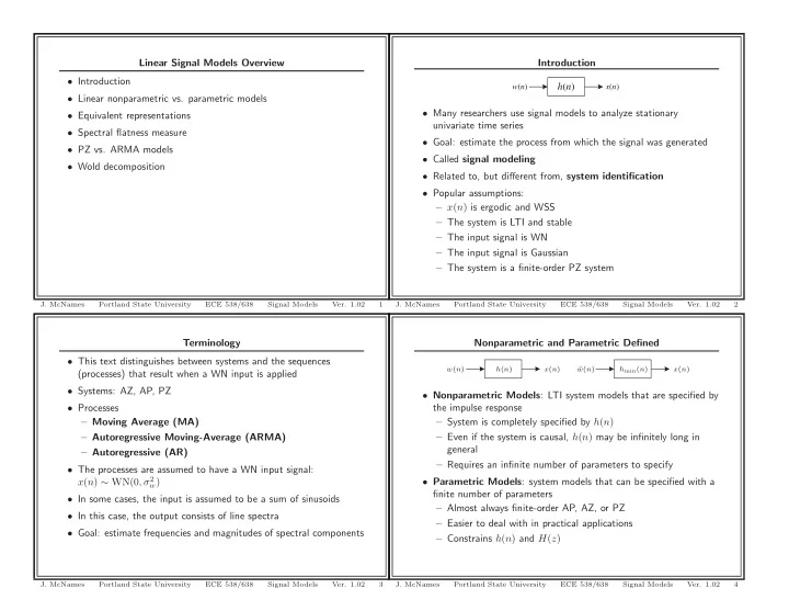
Introduction h(n)

w(n) x(n)

• Many researchers use signal models to analyze stationary

univariate time series

• Goal: estimate the process from which the signal was generated
• Called signal modeling
• Related to, but different from, system identification
• Popular assumptions:

– x(n) is ergodic and WSS – The system is LTI and stable – The input signal is WN – The input signal is Gaussian – The system is a finite-order PZ system

• J. McNames

Portland State University ECE 538/638 Signal Models

• Ver. 1.02

2

SLIDE 2

Nonrecursive Representation h(n)

w(n) x(n)

x(n) =

∞

• k=−∞

h(k)w(n − k) rx(ℓ) = σ2

wrh(ℓ)

Rx(z) = σ2

wH(z)H∗(z−∗)

Rx(ejω) = σ2

w|H(ejω)|2

• Note that this is a non-recursive representation
• Any LTI system can be written in this form
• The shape of rx(ℓ) and Rx(ejω) are completely determined by the

system

• J. McNames

Portland State University ECE 538/638 Signal Models

• Ver. 1.02

7

Nonparametric versus Parametric

• We will focus on nonparametric estimators
• These generally have greater variability but less bias than

parametric estimators. Why?

• However, they do not give a compact representation of the process
• Will discuss parametric models in detail next term
• J. McNames

Portland State University ECE 538/638 Signal Models

• Ver. 1.02

5

Nonrecursive Representation Continued h(n)

w(n) x(n)

x(n) =

∞

• k=0

h(k)w(n − k)

• Since we cannot distinguish between signals produced by causal

and non-causal systems, we can assume the system is causal

• This is identical to an infinite-order (Q = ∞) AZ model!
• We cannot distinguish between the system gain and the white

noise process power: αh(n) ≡ αw(n − k)

• Without loss of generality, we can assume h(0) = 1
• J. McNames

Portland State University ECE 538/638 Signal Models

• Ver. 1.02

8

Why Assume Minimum-Phase? h(n)

w(n) x(n)

• Recall that from Rx(z) alone we cannot distinguish between

minimum and non-minimum-phase systems

• This is true in general
• For any stable, finite-order ARMA process, {H(z), w(n)} where

H(z) has no zeros or poles on the unit circle, there exists a white noise process ˜ w(n) such that X(z) = Hmin(z) ˜ W(z) and Hmin(z) is minimum-phase

• If we have no other information but can only observe the signal,

there is no reason not to assume h(n) is stable and minimum-phase!

• Very important assumption
• If w(n) is IID, it is not true in general that ˜

w(n) is IID

• J. McNames

Portland State University ECE 538/638 Signal Models

• Ver. 1.02

6

SLIDE 3

Comments on Innovations Representation x(n + 1) = w(n + 1)

• New Information

+

n

• k=−∞

h(n + 1 − k) ⎛ ⎝

n

• j=−∞

hI(k − j)x(j) ⎞ ⎠

• Past values of x(n)
• If the system generating x(n) is minimum-phase, w(n + 1) carries

all the new information needed to generate x(n + 1)

• Thus, w(n + 1) is sometimes called the innovation
• All other information can be predicted from past observations of

the output

• Only holds if h(n) is minimum-phase
• In some contexts, h(n) is called the synthesis or coloring filter
• The inverse is called the analysis or whitening filter
• J. McNames

Portland State University ECE 538/638 Signal Models

• Ver. 1.02

11

Recursive Representation h(n)

w(n) x(n)

hI(n)

w(n)

w(n) =

∞

• k=0

hI(k)x(n − k) = x(n) +

∞

• k=1

hI(k)x(n − k) x(n) = w(n) −

∞

• k=1

hI(k)x(n − k)

• Let us choose (without loss of generality) that h(0) = 1
• If we assume the inverse system is causal and stable, then

hI(0) = 1 (why?)

• In this case, the output is a function of the current (unknown)

input and all past values of x(n)

• This is identical to an infinite-order (P = ∞) AP model!
• Equivalent representation of the nonrecursive form
• J. McNames

Portland State University ECE 538/638 Signal Models

• Ver. 1.02

9

PZ, AZ, and AP Representations

• We just saw that a nonparametric model can be represented as

either white noise driving an AZ(∞) system or a PZ(∞) system

• Any causal PZ, AZ, or PZ system with finite order can be

represented as either a causal AZ(∞) or PZ(∞) system

• If the system is stable, then h(n) → 0 as n → ∞
• Thus, if the order of the system is sufficiently large, we can

represent any of these systems accurately with an AZ(Q) or AP(P) system

• We’ll see next term that AP(P) are much easier to estimate than

PZ(Q, P) or AZ(Q) systems

• Thus, it is very good news that AP(P) systems can represent any

PZ(Q, P) or AZ(Q) system if P is large enough

• See Example 4.2.1 in the text and discussion in preceding

paragraph

• J. McNames

Portland State University ECE 538/638 Signal Models

• Ver. 1.02

12

Innovations Representation If we assume H(z) is minimum-phase (reasonable), both h(n) and hI(n) exist and both are causal and stable. x(n) =

∞

• k=0

h(k)w(n − k) =

n

• k=−∞

h(n − k)w(k) x(n + 1) = w(n + 1) +

n

• k=−∞

h(n + 1 − k)w(k) x(n + 1) = w(n + 1)

• New Information

+

n

• k=−∞

h(n + 1 − k) ⎛ ⎝

n

• j=−∞

hI(k − j)x(j) ⎞ ⎠

• Past values of x(n)
• J. McNames

Portland State University ECE 538/638 Signal Models

• Ver. 1.02

10

SLIDE 4

Spectral Flatness SFMx exp

• 1

2π

π

−π ln

• Rx(ejω)
• dω
• 1

2π

π

−π Rx(ejω) dω

= σ2

w

σ2

x

• Single measure of the spectral flatness
• Bounded:

0 ≤ SFMx ≤ 1

• If SFMx = 1, then x(n) is a white process
• Numerator is the geometric mean, denominator is the arithmetic

mean

• J. McNames

Portland State University ECE 538/638 Signal Models

• Ver. 1.02

15

Spectral Factorization Rx(ejω) = σ2

w|Hmin(ejω)|2

• Regular: Processes that satisfy the Paley-Wiener condition

π

−π

| ln Rx(ejω)|dω < ∞

• Regular processes can be factored as

Rx(z) = σ2

wHmin(z)H∗ min(z−∗)

σ2

w = exp

1 2π π

−π

ln

• Rx(ejω)
• dω
• J. McNames

Portland State University ECE 538/638 Signal Models

• Ver. 1.02

13

Parametric Signal Models

P

• k=0

akx(n − k) =

Q

• k=0

bkw(n − k) H(z) = X(z) W(z) = Q

k=0 bkz−k

P

k=0 akz−k = B(z)

A(z)

• Parametric models have rational (finite-order) system functions
• Each can be specified by a linear constant-coefficient difference

equation

• To make the specifications unique, we always set a0 = 1 and

usually b0 = 1

• The model is then defined by {a1, a2, . . . , aP , b1, . . . , bQ, σ2

w}

• J. McNames

Portland State University ECE 538/638 Signal Models

• Ver. 1.02

16

Cepstrum The cepstrum is the inverse Fourier transform of ln Rx(ejω) c(k) 1 2π π

−π

ln

• Rx(ejω)
• ejkωdω
• The minimum-phase component of the spectrum is the causal part

c+(k) 1

2c(0) + c(k)u(k − 1)

hmin(n) = F−1 {exp F {c+(k)}}

• The maximum-phase component is the anticausal part

c−(k) 1

2c(0) + c(k)u(−k − 1)

hmax(n) = F−1 {exp F {c−(k)}}

• This is rarely used in practice.
• If Rx(z) is a rational function, spectral factorization is

straightforward

• J. McNames

Portland State University ECE 538/638 Signal Models

• Ver. 1.02

14

SLIDE 5

Parametric Signal Model Theory h(n)

w(n) x(n)

hI(n)

w(n)

• There are many equivalent representations of WSS processes

modeled as WN driving an LTI system – Impulse response h(n) and σ2

w

– Inverse system impulse response hI(n) and σ2

w

– Output autocorrelation – Output PSD Rx(ejω)

• If we assume a parametric model, we can also specify by

{a1, a2, . . . , aP , b1, . . . , bQ, σ2

w}

• If we consider lattice filters, we have yet another representation
• All are complete descriptions of the processes
• J. McNames

Portland State University ECE 538/638 Signal Models

• Ver. 1.02

19

Parametric Signal Models x(n) +

P

• k=1

akx(n − k) = w(n) +

Q

• k=1

bkw(n − k) H(z) = X(z) W(z) = 1 + Q

k=1 bkz−k

1 + P

k=1 akz−k = B(z)

A(z)

• The models are generally divided into three categories

– Moving-Average Model: MA(Q), P = 0 – Autoregressive Model: AR(P), Q = 0 – Autoregressive Moving-Average Model: ARMA(P,Q)

• All models assume the systems are BIBO stable
• In general, when estimating, we constrain ourselves to

minimum-phase systems

• J. McNames

Portland State University ECE 538/638 Signal Models

• Ver. 1.02

17

WOLD Decomposition WOLD Decomposition: A general stationary random process can be written as x(n) = xr(n) + xp(n) where xr(n) is a regular process with a continuous PSD and xp(n) is a predictable process with a discrete

• spectrum. Further

E

• xr(n1)x∗

p(n2)

• = 0

∀n1, n2

• In general, stationary random processes consist of a continuous

PSD Rx(ejω) and a discrete power spectrum with DTFS coefficients Rx(k)

• These processes are called mixed
• Continuous PSD is due to regular processes (unpredictable)
• Discrete is due to harmonic or almost periodic processes

(predictable)

• The autocorrelation is rx(ℓ) = rxr(ℓ) + rxp(ℓ)
• Proof is very difficult (see references in text)
• J. McNames

Portland State University ECE 538/638 Signal Models

• Ver. 1.02

20

Parametric Signal Model Limitations x(n) +

P

• k=1

akx(n − k) = w(n) +

Q

• k=1

bkw(n − k) H(z) = X(z) W(z) = 1 + Q

k=1 bkz−k

1 + P

k=1 akz−k = B(z)

A(z)

• Parametric signal models all have short-memory behavior
• The autocorrelation decays exponentially
• AZ systems can have any impulse response (unconstrained)
• AP and PZ systems are constrained because the poles must be

inside the unit circle – Long-term behavior is a sum of decaying exponentials

• Parametric models are useful for creating processes with any

continuous spectrum (PSD)

• J. McNames

Portland State University ECE 538/638 Signal Models

• Ver. 1.02

18