Parallelised Bayesian Optimisation via Thompson Sampling - PowerPoint PPT Presentation
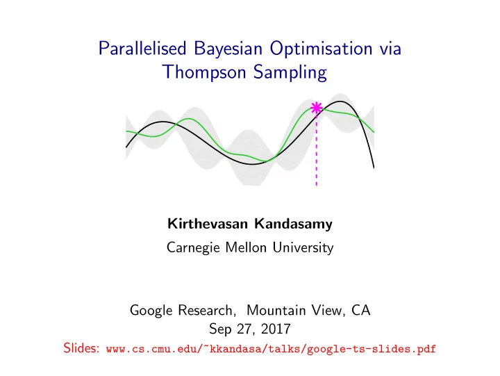
Parallelised Bayesian Optimisation via Thompson Sampling Kirthevasan Kandasamy Carnegie Mellon University Google Research, Mountain View, CA Sep 27, 2017 Slides: www.cs.cmu.edu/~kkandasa/talks/google-ts-slides.pdf www.cs.cmu.edu/ kkandasa
Big picture: scaling up black-box optimisation ◮ Optimising in high dimensional spaces e.g.: Tuning models with several hyper-parameters Additive models for f lead to statistically and computationally tractable algorithms. (Kandasamy et al. ICML 2015) ◮ Multi-fidelity optimisation: what if we have cheap approximations to f ? E.g. Train an ML model with N • data and T • iterations. But use N < N • data and T < T • iterations to approximate cross validation performance at ( N • , T • ). (Kandasamy et al. NIPS 2016a&b, Kandasamy et al. ICML 2017) Extends beyond GPs. 9/31
This work: Parallel Evaluations (Kandasamy et al. Arxiv 2017) Parallelisation with M workers: can evaluate f at M different points at the same time. E.g. Train M models with different hyper-parameter values in parallel at the same time. Inability to parallelise is a real bottleneck in practice! 10/31
This work: Parallel Evaluations (Kandasamy et al. Arxiv 2017) Parallelisation with M workers: can evaluate f at M different points at the same time. E.g. Train M models with different hyper-parameter values in parallel at the same time. Inability to parallelise is a real bottleneck in practice! Some desiderata: ◮ Statistically, achieve × M improvement. ◮ Methodologically, be scalable for a very large number of workers, - Method remains computationally tractable as M increases. - Method is conceptually simple, for robustness in practice. 10/31
Outline (Kandasamy et al. Arxiv 2017) 1. Set up & definitions 2. Prior work & challenges 3. Algorithms synTS , asyTS : direct application of TS to synchronous and asynchronous parallel settings 4. Experiments 5. Theoretical Results 6. Open questions/challenges 11/31
Outline (Kandasamy et al. Arxiv 2017) 1. Set up & definitions 2. Prior work & challenges 3. Algorithms synTS , asyTS : direct application of TS to synchronous and asynchronous parallel settings 4. Experiments 5. Theoretical Results ◮ synTS and asyTS perform essentially the same as seqTS in terms of the number of evaluations. ◮ When we factor time as a resource, asyTS outperforms synTS and seqTS . . . . with some caveats. 6. Open questions/challenges 11/31
Outline (Kandasamy et al. Arxiv 2017) 1. Set up & definitions 2. Prior work & challenges 3. Algorithms synTS , asyTS : direct application of TS to synchronous and asynchronous parallel settings 4. Experiments 5. Theoretical Results ◮ synTS and asyTS perform essentially the same as seqTS in terms of the number of evaluations. ◮ When we factor time as a resource, asyTS outperforms synTS and seqTS . . . . with some caveats 6. Open questions/challenges 11/31
Parallel Evaluations: set up Sequential evaluations with one worker 12/31
Parallel Evaluations: set up Sequential evaluations with one worker Parallel evaluations with M workers (Asynchronous) 12/31
Parallel Evaluations: set up Sequential evaluations with one worker Parallel evaluations with M workers (Asynchronous) Parallel evaluations with M workers (Synchronous) 12/31
Parallel Evaluations: set up Sequential evaluations with one worker j th job has feedback from all previous j − 1 jobs. Parallel evaluations with M workers (Asynchronous) j th job missing feedback from exactly M − 1 jobs. Parallel evaluations with M workers (Synchronous) j th job missing feedback from ≤ M − 1 jobs. 12/31
Simple Regret in Parallel Settings (Kandasamy et al. Arxiv 2017) Simple regret after n evaluations , SR( n ) = f ( x ⋆ ) − max t =1 ,..., n f ( x t ) . n ← number of completed evaluations by all M workers. 13/31
Simple Regret in Parallel Settings (Kandasamy et al. Arxiv 2017) Simple regret after n evaluations , SR( n ) = f ( x ⋆ ) − max t =1 ,..., n f ( x t ) . n ← number of completed evaluations by all M workers. Simple regret with time as a resource , Asynchronous Synchronous SR ′ ( T ) = f ( x ⋆ ) − t =1 ,..., N f ( x t ) . max N ← (possibly random) number of completed evaluations by all M workers within time T . 13/31
Outline (Kandasamy et al. Arxiv 2017) 1. Set up & definitions 2. Prior work & challenges 3. Algorithms synTS , asyTS : direct application of TS to synchronous and asynchronous parallel settings 4. Experiments 5. Theoretical Results ◮ synTS and asyTS perform essentially the same as seqTS in terms of the number of evaluations. ◮ When we factor time as a resource, asyTS outperforms synTS and seqTS . . . . with some caveats 6. Open questions/challenges 13/31
Prior work in Parallel BO (Ginsbourger et al. 2011) (Janusevkis et al. 2012) (Contal et al. 2013) (Desautels et al. 2014) (Gonzalez et al. 2015) (Shah & Ghahramani. 2015) (Wang et al. 2016) (Kathuria et al. 2016) (Wu & Frazier. 2017) (Wang et al. 2017) (Kandasamy et al. Arxiv 2017) 14/31
Prior work in Parallel BO Asynchr- onicity � (Ginsbourger et al. 2011) � (Janusevkis et al. 2012) (Contal et al. 2013) (Desautels et al. 2014) (Gonzalez et al. 2015) (Shah & Ghahramani. 2015) � (Wang et al. 2016) (Kathuria et al. 2016) (Wu & Frazier. 2017) (Wang et al. 2017) � (Kandasamy et al. Arxiv 2017) 14/31
Prior work in Parallel BO Asynchr- Theoretical onicity guarantees � (Ginsbourger et al. 2011) � (Janusevkis et al. 2012) � (Contal et al. 2013) � (Desautels et al. 2014) (Gonzalez et al. 2015) (Shah & Ghahramani. 2015) � (Wang et al. 2016) � (Kathuria et al. 2016) (Wu & Frazier. 2017) (Wang et al. 2017) � � (Kandasamy et al. Arxiv 2017) 14/31
Prior work in Parallel BO Asynchr- Theoretical Conceptual onicity guarantees simplicity * � (Ginsbourger et al. 2011) � (Janusevkis et al. 2012) � (Contal et al. 2013) � (Desautels et al. 2014) (Gonzalez et al. 2015) (Shah & Ghahramani. 2015) � (Wang et al. 2016) � (Kathuria et al. 2016) (Wu & Frazier. 2017) (Wang et al. 2017) � � � (Kandasamy et al. Arxiv 2017) * straightforward extension of sequential algorithm works. 14/31
Why are deterministic algorithms not “simple”? Need to encourage diversity in parallel evaluations Direct application of GP-UCB in the synchronous setting ... f ( x ) x 15/31
Why are deterministic algorithms not “simple”? Need to encourage diversity in parallel evaluations Direct application of GP-UCB in the synchronous setting ... - First worker: maximise acquisition, x t 1 = argmax ϕ t ( x ). ϕ t = µ t − 1 + β 1 / 2 f ( x ) σ t − 1 t x t 1 x 15/31
Why are deterministic algorithms not “simple”? Need to encourage diversity in parallel evaluations Direct application of GP-UCB in the synchronous setting ... - First worker: maximise acquisition, x t 1 = argmax ϕ t ( x ). - Second worker: acquisition is the same! x t 1 = x t 2 ϕ t = µ t − 1 + β 1 / 2 f ( x ) σ t − 1 t x t 2 = x t 1 x 15/31
Why are deterministic algorithms not “simple”? Need to encourage diversity in parallel evaluations Direct application of GP-UCB in the synchronous setting ... - First worker: maximise acquisition, x t 1 = argmax ϕ t ( x ). - Second worker: acquisition is the same! x t 1 = x t 2 - x t 1 = x t 2 = · · · = x tM . ϕ t = µ t − 1 + β 1 / 2 f ( x ) σ t − 1 t x t 2 = x t 1 x 15/31
Why are deterministic algorithms not “simple”? Need to encourage diversity in parallel evaluations Direct application of GP-UCB in the synchronous setting ... - First worker: maximise acquisition, x t 1 = argmax ϕ t ( x ). - Second worker: acquisition is the same! x t 1 = x t 2 - x t 1 = x t 2 = · · · = x tM . ϕ t = µ t − 1 + β 1 / 2 f ( x ) σ t − 1 t x t 2 = x t 1 x Direct application of sequential algorithm does not work. Need to “encourage diversity”. 15/31
Why are deterministic algorithms not “simple”? Need to encourage diversity in parallel evaluations ◮ Add hallucinated observations. f ( x ) x 16/31
Why are deterministic algorithms not “simple”? Need to encourage diversity in parallel evaluations ◮ Add hallucinated observations. f ( x ) ˆ f x 16/31
Why are deterministic algorithms not “simple”? Need to encourage diversity in parallel evaluations ◮ Add hallucinated observations. f ( x ) ˆ f x 16/31
Why are deterministic algorithms not “simple”? Need to encourage diversity in parallel evaluations ◮ Add hallucinated observations. f ( x ) x 16/31
Why are deterministic algorithms not “simple”? Need to encourage diversity in parallel evaluations ◮ Add hallucinated observations. f ( x ) x ◮ Optimise an acquisition over X M . 16/31
Why are deterministic algorithms not “simple”? Need to encourage diversity in parallel evaluations ◮ Add hallucinated observations. f ( x ) x ◮ Optimise an acquisition over X M . ◮ Resort to heuristics, typically requires additional hyper-parameters and/or computational routines. 16/31
Why are deterministic algorithms not “simple”? Need to encourage diversity in parallel evaluations ◮ Add hallucinated observations. f ( x ) x ◮ Optimise an acquisition over X M . ◮ Resort to heuristics, typically requires additional hyper-parameters and/or computational routines. Take-home message: Straightforward application of sequential algorithm works for TS. Inherent randomness takes care of exploration vs. exploitation trade-off when managing M workers. 16/31
Parallel Thompson Sampling (Kandasamy et al. Arxiv 2017) Asynchronous: asyTS At any given time, 1. ( x ′ , y ′ ) ← Wait for a worker to finish. 2. Compute posterior GP . 3. Draw a sample g ∼ GP . 4. Re-deploy worker at argmax g . 17/31
Parallel Thompson Sampling (Kandasamy et al. Arxiv 2017) Synchronous: synTS Asynchronous: asyTS At any given time, At any given time, 1. { ( x ′ m , y ′ 1. ( x ′ , y ′ ) ← Wait for m ) } M m =1 ← Wait for a worker to finish. all workers to finish. 2. Compute posterior GP . 2. Compute posterior GP . 3. Draw a sample g ∼ GP . 3. Draw M samples g m ∼ GP , ∀ m . 4. Re-deploy worker at 4. Re-deploy worker m at argmax g m , ∀ m . argmax g . 17/31
Parallel Thompson Sampling (Kandasamy et al. Arxiv 2017) Synchronous: synTS Asynchronous: asyTS At any given time, At any given time, 1. { ( x ′ m , y ′ 1. ( x ′ , y ′ ) ← Wait for m ) } M m =1 ← Wait for a worker to finish. all workers to finish. 2. Compute posterior GP . 2. Compute posterior GP . 3. Draw a sample g ∼ GP . 3. Draw M samples g m ∼ GP , ∀ m . 4. Re-deploy worker at 4. Re-deploy worker m at argmax g m , ∀ m . argmax g . Variants in prior work: (Osband et al. 2016, Israelsen et al. 2016, Hernandez-Lobato et al. 2017) 17/31
Outline (Kandasamy et al. Arxiv 2017) 1. Set up & definitions 2. Prior work & challenges 3. Algorithms synTS , asyTS : direct application of TS to synchronous and asynchronous parallel settings 4. Experiments 5. Theoretical Results ◮ synTS and asyTS perform essentially the same as seqTS in terms of the number of evaluations. ◮ When we factor time as a resource, asyTS outperforms synTS and seqTS . . . . with some caveats 6. Open questions/challenges 18/31
Experiment: Park1-4D M = 10 Comparison in terms of number of evaluations 10 0 asyTS synTS seqTS 0 20 40 60 80 100 120 19/31
Experiment: Branin-2D M = 4 Evaluation time sampled from a uniform distribution 10 -1 10 -2 0 10 20 30 40 20/31
Experiment: Branin-2D M = 4 Evaluation time sampled from a uniform distribution 10 -1 10 -2 0 10 20 30 40 20/31
Experiment: Branin-2D M = 4 Evaluation time sampled from a uniform distribution synRAND synHUCB synUCBPE synTS 10 -1 asyRAND asyUCB asyHUCB asyEI asyHTS 10 -2 asyTS 0 10 20 30 40 20/31
Experiment: Hartmann-6D M = 12 Evaluation time sampled from a half-normal distribution synRAND synHUCB 10 0 synUCBPE synTS asyRAND asyUCB asyHUCB asyEI asyHTS asyTS 10 -1 0 5 10 15 20 25 30 21/31
Experiment: Hartmann-18D M = 25 Evaluation time sampled from an exponential distribution synRAND 6.5 synHUCB 6 synUCBPE 5.5 synTS 5 asyRAND 4.5 asyUCB 4 asyHUCB asyEI 3.5 asyHTS asyTS 3 2.5 0 5 10 15 20 25 30 22/31
Experiment: Currin-Exponential-14D M = 35 Evaluation time sampled from a Pareto-3 distribution synRAND synHUCB 25 synUCBPE synTS 20 asyRAND asyUCB asyHUCB asyEI 15 asyHTS asyTS 10 0 5 10 15 20 23/31
Experiment: Model Selection in Cifar10 M = 4 Tune # filters in in range (32 , 256) for each layer in a 6 layer CNN. Time taken for an evaluation: 4 - 16 minutes. asyTS 0.72 asyEI 0.71 asyHUCB asyRAND synTS 0.7 0.69 synHUCB 0.68 1000 2000 3000 4000 5000 6000 7000 24/31
Outline (Kandasamy et al. Arxiv 2017) 1. Set up & definitions 2. Prior work & challenges 3. Algorithms synTS , asyTS : direct application of TS to synchronous and asynchronous parallel settings 4. Experiments 5. Theoretical Results ◮ synTS and asyTS perform essentially the same as seqTS in terms of the number of evaluations. ◮ When we factor time as a resource, asyTS outperforms synTS and seqTS . . . . with some caveats. 6. Open questions/challenges 24/31
Bounds for SR( n ), synTS seqTS (Russo & van Roy 2014) � Ψ n log( n ) E [SR( n )] � n Ψ n ← Maximum information gain. 25/31
Bounds for SR( n ), synTS seqTS (Russo & van Roy 2014) � Ψ n log( n ) E [SR( n )] � n Ψ n ← Maximum information gain. Theorem: synTS (Kandasamy et al. Arxiv 2017) � � log( M ) E [SR( n )] � M Ψ n + M log( n + M ) + n n Leading constant is also the same. 25/31
Bounds for SR( n ), asyTS seqTS (Russo & van Roy 2014) � Ψ n log( n ) E [SR( n )] � n 26/31
Bounds for SR( n ), asyTS seqTS (Russo & van Roy 2014) � Ψ n log( n ) E [SR( n )] � n Theorem: asyTS (Kandasamy et al. Arxiv 2017) � ξ M Ψ n log( n ) E [SR( n )] � n ξ M = sup D n , n ≥ 1 max A ⊂X , | A |≤ M e I ( f ; A |D n ) . 26/31
Bounds for SR( n ), asyTS seqTS (Russo & van Roy 2014) � Ψ n log( n ) E [SR( n )] � n Theorem: asyTS (Kandasamy et al. Arxiv 2017) � ξ M Ψ n log( n ) E [SR( n )] � n ξ M = sup D n , n ≥ 1 max A ⊂X , | A |≤ M e I ( f ; A |D n ) . Theorem: There exists an asynchronously parallelisable initiali- sation scheme requiring O ( M polylog ( M )) evaluations to f such that ξ M ≤ C . (Krause et al. 2008, Desautels et al. 2012) 26/31
Bounds for SR( n ), asyTS seqTS (Russo & van Roy 2014) � Ψ n log( n ) E [SR( n )] � n Theorem: asyTS , arbitrary X (Kandasamy et al. Arxiv 2017) � E [SR( n )] � M polylog ( M ) C Ψ n log( n ) + n n ξ M = sup D n , n ≥ 1 max A ⊂X , | A |≤ M e I ( f ; A |D n ) . Theorem: There exists an asynchronously parallelisable initiali- sation scheme requiring O ( M polylog ( M )) evaluations to f such that ξ M ≤ C . (Krause et al. 2008, Desautels et al. 2012) 26/31
Bounds for SR( n ), asyTS seqTS (Russo & van Roy 2014) � Ψ n log( n ) E [SR( n )] � n Theorem: asyTS , arbitrary X (Kandasamy et al. Arxiv 2017) � E [SR( n )] � M polylog ( M ) C Ψ n log( n ) + n n ξ M = sup D n , n ≥ 1 max A ⊂X , | A |≤ M e I ( f ; A |D n ) . Theorem: There exists an asynchronously parallelisable initiali- sation scheme requiring O ( M polylog ( M )) evaluations to f such that ξ M ≤ C . (Krause et al. 2008, Desautels et al. 2012) * We do not believe this is necessary. 26/31
Bounds for asyTS without the initialisation scheme Theorem: synTS , arbitrary X (Kandasamy et al. Arxiv 2017) � � E [SR( n )] � M log( M ) Ψ n + M log( n + M ) + n n 27/31
Bounds for asyTS without the initialisation scheme Theorem: synTS , arbitrary X (Kandasamy et al. Arxiv 2017) � � E [SR( n )] � M log( M ) Ψ n + M log( n + M ) + n n Theorem: asyTS , X ⊂ R d (Ongoing work) � M log( n ) E [SR( n )] � . . . + n 1 / O ( d ) 27/31
Theoretical Results for SR ′ ( T ) Model evaluation time as an independent random variable ◮ Uniform unif( a , b ) bounded HN ( τ 2 ) ◮ Half-normal sub-Gaussian ◮ Exponential exp( λ ) sub-exponential 28/31
Recommend


More recommend
Explore More Topics
Stay informed with curated content and fresh updates.